Power to detect mediation and other problems
September 2, 2016
I was reminded of this old R Club post recently by Rose, and decided to flesh it out a bit. The first part is about power to detect mediation in the standard 3 variable model people use. The second part examines how model misspecification gives rise to significant statistical tests of mediation when there is actually no mediation going on. Since publishing a paper (in press now, but written in ~2013) in which longitudinal data was subjected to a test of mediation, I’ve become increasingly skeptical of these kinds of analyses (including my own).
If you haven’t read this article by John Bullock and colleagues, you really, really should. The tl;dr is that mediation is always a claim about a chain of causation, and since causation itself is very difficult to pin down, mediation is doubly so. It’s a great read, and a necessary starting place if you’re serious about pursuing research on mediating processes.
Bullock, J. G., Green, D. P., & Ha, S. E. (2010). Yes, but what’s the mechanism? (don’t expect an easy answer). Journal of Personality and Social Psychology, 98(4), 550–558. http://doi.org/10.1037/a0018933
You’ll also probably want to check out docs for
Power
We’ll start as usual by loading packages – uncomment the install.pacakges lines if you don’t have them.
#install.packages('lavaan')
library(lavaan)
#install.packages('semPlot')
library(semPlot)
#install.packages('simsem')
library(simsem)
#install.packages('dplyr')
library(dplyr)
#install.packages('ggplot2')
library(ggplot2)
library(knitr)
In the next step, we set the effect sizes for which we want to compute power, and generate a bunch of lavaan model syntax that will subsequently let us simulate data based on these effect sizes.
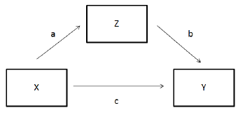
The variable and path names corresond roughly to this diagram (I switched between using Z and M for the mediator variable).
effectSizes <- c(.1,  .3, .5)

modelEffects <- expand.grid(effectSizes, effectSizes, effectSizes)
names(modelEffects) <- c('a', 'b', 'c')

# generate data (genModel) and then test the model (testModel)
# if we want 80% power than in 80% of simulations we should find an effect

models <- modelEffects %>%
    rowwise() %>%
    do({
        genModel <- paste0('# direct effect
                           Y ~ ', .$c, '*X
                           # mediator
                           M ~ ', .$a, '*X
                           Y ~ ', .$b, '*M
                           X ~~ 1*X
                           Y ~~ 1*Y
                           M ~~ 1*M
                           ')
        testModel <-'# direct effect
                    Y ~ c*X
                    # mediator
                    M ~ a*X
                    Y ~ b*M
                    # indirect effect (a*b)
                    ab := a*b
                    # total effect
                    total := c + (a*b)
                    '
        data.frame(a=.$a, b=.$b, c=.$c,
                   gen=genModel, test=testModel, stringsAsFactors=F)
    })
The testModel above is the model we’ll estimate. Notice that it’s equivalent in structure to that which is generating the data. We’re not worrying about model misspecification at this point.
We now have a data structure, in models, representing all combinations of the effect sizes, and we can run each of them at different sample sizes using the simsem package. Like most simulations, it’s probably a good idea to save the output so you don’t have to slog through the simulations again. You should set REDOSIMS=T below to run them the first time. Using 8 threads on a fairly modern machine takes about 10 minutes.
The steps below are roughly:
- Within each level combination of
a,b, andceffect sizes, - for every sample size from 50 to 1500:
- generate simulated data and estimate a model on those data.
REDOSIMS=F
if(REDOSIMS){
    allModelPowerSim <- models %>%
        rowwise() %>%
        do({
            manySims <- sim(NULL, model=.$test[1], n=50:1500, generate=.$gen[1],
                            lavaanfun='sem', multicore=T) # Enable multicore on your personal computer
            data_frame(a=.$a, b=.$b, c=.$c, powersims=list(manySims))
        })
        #saving the above
        saveRDS(allModelPowerSim, 'power_simulations.RDS')
} else {
    #loading the above
    allModelPowerSim <- readRDS('power_simulations.RDS')
}
Next, we’ll estimate the $\text{power}(\text{sample size})$ function to detect a significant a*b path for each of our levels of the effect sizes for the 3 paths.
powerData <- allModelPowerSim %>% rowwise() %>%
    do({
        aSimPower <- as.data.frame(getPower(.$powersims,
                                            nVal=seq(50, 1500, 5),
                                            powerParam='ab'))
        data_frame(a=.$a, b=.$b, c=.$c,
                   alab=paste0('a=',.$a),
                   blab=paste0('b=',.$b),
                   clab=paste0('c=',.$c),
                   N=aSimPower[,1],
                   ab=aSimPower[,2])
    })

print(powerData)
## Source: local data frame [7,857 x 8]
## Groups: <by row>
##
## # A tibble: 7,857 × 8
##        a     b     c  alab  blab  clab     N         ab
## *  <dbl> <dbl> <dbl> <chr> <chr> <chr> <dbl>      <dbl>
## 1    0.1   0.1   0.1 a=0.1 b=0.1 c=0.1    50 0.03226034
## 2    0.1   0.1   0.1 a=0.1 b=0.1 c=0.1    55 0.03284883
## 3    0.1   0.1   0.1 a=0.1 b=0.1 c=0.1    60 0.03344768
## 4    0.1   0.1   0.1 a=0.1 b=0.1 c=0.1    65 0.03405707
## 5    0.1   0.1   0.1 a=0.1 b=0.1 c=0.1    70 0.03467715
## 6    0.1   0.1   0.1 a=0.1 b=0.1 c=0.1    75 0.03530812
## 7    0.1   0.1   0.1 a=0.1 b=0.1 c=0.1    80 0.03595014
## 8    0.1   0.1   0.1 a=0.1 b=0.1 c=0.1    85 0.03660339
## 9    0.1   0.1   0.1 a=0.1 b=0.1 c=0.1    90 0.03726805
## 10   0.1   0.1   0.1 a=0.1 b=0.1 c=0.1    95 0.03794431
## # ... with 7,847 more rows
This produces a 7,857-row table (er, tibble). Sounds like something better to plot:
ggplot(powerData, aes(x=N, y=ab))+
    geom_line(aes(color=clab),alpha=.7, size=1)+
    facet_grid(alab ~ blab, as.table=F)+
    geom_hline(yintercept=.8,color='red',alpha=.5)+
    labs(x='sample size', y='power to detect a*b', color='direct effect')
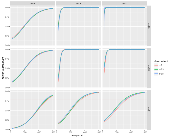
And we can get the sample size for 80% power to detect an effect at any of our levels. As an example, let’s take the first row from allModelPowerSims:
allModelPowerSim[1,]
## # A tibble: 1 × 4
##       a     b     c       powersims
##   <dbl> <dbl> <dbl>          <list>
## 1   0.1   0.1   0.1 <S4: SimResult>
aPowerTable <- getPower(allModelPowerSim$powersims[[1]])
#?findPower
findPower(aPowerTable,
          iv="N",
          power=.8)
##     c     a     b  Y~~Y  M~~M    ab total
##   809   837   858   Inf   Inf  1332   687
So, for a small effect for paths a and b, you need 1,332 participants for 80% power (and if you want to know why you should think about small effects, read this).
When I first presented this in R club, I left the below as an exercise:
Go ahead and make a data table of the power for finding the true mediated effect, ab, at each effect size level using ‘do’, below.
abPower80 <- allModelPowerSim %>%
    group_by(a, b, c) %>%
    do({
        aPowerTable <- getPower()
        theNfor80percPower <- findPower()
        data.frame()
    })
The c path doesn’t have much of an effect, so I left it out. Hopefully, you got something like this:
| a | b | c | N_for_ab |
|---|---|---|---|
| 0.1 | 0.1 | 0.3 | 1297 |
| 0.1 | 0.3 | 0.3 | 842 |
| 0.1 | 0.5 | 0.3 | 786 |
| 0.3 | 0.1 | 0.3 | 858 |
| 0.3 | 0.3 | 0.3 | 151 |
| 0.3 | 0.5 | 0.3 | 102 |
| 0.5 | 0.1 | 0.3 | 862 |
| 0.5 | 0.3 | 0.3 | 110 |
| 0.5 | 0.5 | 0.3 | 51 |
Misspecification
As I mentioned in the preamble, statistical mediation relies on a certain model of causal processes. What happens if the true process that gives rise to your observed data doesn’t conform to the simple mediation model? Using lavaan and simsem, it’s easy to generate data from one model and analyze it (repeatedly) with another. Mediation, being causal, necessitates the use of longitudinal data. According to Todd Little, two waves is enough assuming you have the model right[citation needed].
So our data generating model will use 3 variables measured twice: X, Y, and Z – the independent, dependent, and mediator respectively. These three variables will be highly stable (test-retest between the two waves of r=.7), and moderately correlated with each other at r=.3. Importantly, we’re going to generate data in which there is absolutely no causal effect between the three variables.
generatingModel <- '
y2 ~ .7*y1
x2 ~ .7*x1
z2 ~ .7*z1
y1 ~~ .3*x1 + .3*z1
x1 ~~ .3*z1
y2 ~~ .3*x2 + .3*z2
x2 ~~ .3*z2
y2 ~ 0*x1 + 0*z1
x2 ~ 0*y1 + 0*z1
z2 ~ 0*y1 + 0*x1
y1 ~~ 1*y1
x1 ~~ 1*x1
z1 ~~ 1*z1
y2 ~~ 1*y2
x2 ~~ 1*x2
z2 ~~ 1*z2
'
We can check out a few misspecifications. First, we’ll test the best case scenario short of testing the true model. In mediationModelControlzT1 we do the usual longitudinal best-practice of regressing our wave 2 dependent variable on its wave 1 measurement (y2 ~ y1 + c*x1 + b*z2). In the regression of our wave 2 mediator on the independent variable, we can also include the mediator’s wave 1 measurement (z2 ~ a*x1 + z1). Conceptually, we’ve made sure to account for stability within each variable over time – most simple models of mediation don’t do this.
In the two other misspecified models, we additionally leave out the measurement of the mediator at wave 1, and then also leave out the measurement of the dependent variable at wave 1.
mediationModelControlzT1 <- '# direct effect
y2 ~ y1 + c*x1 + b*z2
z2 ~ a*x1 + z1
# indirect effect (a*b)
ab := a*b
# total effect
total := c + (a*b)
'
mediationModelNoControlzT1 <- '# direct effect
y2 ~ y1 + c*x1 + b*z2
z2 ~ a*x1
# indirect effect (a*b)
ab := a*b
# total effect
total := c + (a*b)
'
mediationModelNoControlzOryT1 <- '# direct effect
y2 ~ c*x1 + b*z2
z2 ~ a*x1
# indirect effect (a*b)
ab := a*b
# total effect
total := c + (a*b)
'
Before running a buch of simulations, I’ll make sure the models are as expected by generating a single set, and fitting the above.
someData <- simulateData(model=generatingModel, sample.nobs=250, empirical=T)
fit.DGM <- sem(generatingModel, someData, fixed.x=F)
fit.CtrlT1.yz <- sem(mediationModelControlzT1, someData)
fit.noCtrlT1.z <- sem(mediationModelNoControlzT1, someData)
fit.noCtrlT1.yz <- sem(mediationModelNoControlzOryT1, someData)
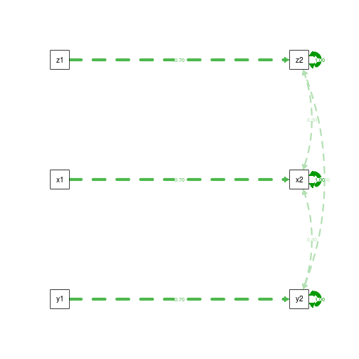
First, the data generating model:
summary(fit.DGM)
## ** WARNING ** lavaan (0.5-20) model has NOT been fitted
## ** WARNING ** Estimates below are simply the starting values
##
##   Number of observations                           250
##
##   Estimator                                         ML
##   Minimum Function Test Statistic                   NA
##   Degrees of freedom                                NA
##   P-value                                           NA
##
## Parameter Estimates:
##
##   Information                                 Expected
##   Standard Errors                             Standard
##
## Regressions:
##                    Estimate  Std.Err  Z-value  P(>|z|)
##   y2 ~
##     y1                0.700
##   x2 ~
##     x1                0.700
##   z2 ~
##     z1                0.700
##   y2 ~
##     x1                0.000
##     z1                0.000
##   x2 ~
##     y1                0.000
##     z1                0.000
##   z2 ~
##     y1                0.000
##     x1                0.000
##
## Covariances:
##                    Estimate  Std.Err  Z-value  P(>|z|)
##   y1 ~~
##     x1                0.300
##     z1                0.300
##   x1 ~~
##     z1                0.300
##   y2 ~~
##     x2                0.300
##     z2                0.300
##   x2 ~~
##     z2                0.300
##
## Variances:
##                    Estimate  Std.Err  Z-value  P(>|z|)
##     y1                1.000
##     x1                1.000
##     z1                1.000
##     y2                1.000
##     x2                1.000
##     z2                1.000
semPaths(fit.DGM, what='est', rotation=2, exoCov=F, exoVar=F)
Next, our best shot, controlling for the mediator and dependent variable at wave 1.
summary(fit.CtrlT1.yz)
## lavaan (0.5-20) converged normally after  12 iterations
##
##   Number of observations                           250
##
##   Estimator                                         ML
##   Minimum Function Test Statistic                7.234
##   Degrees of freedom                                 2
##   P-value (Chi-square)                           0.027
##
## Parameter Estimates:
##
##   Information                                 Expected
##   Standard Errors                             Standard
##
## Regressions:
##                    Estimate  Std.Err  Z-value  P(>|z|)
##   y2 ~
##     y1                0.666    0.065   10.292    0.000
##     x1         (c)   -0.034    0.065   -0.527    0.598
##     z2         (b)    0.211    0.051    4.110    0.000
##   z2 ~
##     x1         (a)    0.000    0.066    0.000    1.000
##     z1                0.700    0.066   10.558    0.000
##
## Variances:
##                    Estimate  Std.Err  Z-value  P(>|z|)
##     y2                0.937    0.084   11.180    0.000
##     z2                1.000    0.089   11.180    0.000
##
## Defined Parameters:
##                    Estimate  Std.Err  Z-value  P(>|z|)
##     ab                0.000    0.014    0.000    1.000
##     total            -0.034    0.066   -0.515    0.607
semPaths(fit.CtrlT1.yz, what='est', rotation=2, exoCov=F, exoVar=F)
Now, progressively leaving things out….
summary(fit.noCtrlT1.z)
## lavaan (0.5-20) converged normally after  12 iterations
##
##   Number of observations                           250
##
##   Estimator                                         ML
##   Minimum Function Test Statistic                4.140
##   Degrees of freedom                                 1
##   P-value (Chi-square)                           0.042
##
## Parameter Estimates:
##
##   Information                                 Expected
##   Standard Errors                             Standard
##
## Regressions:
##                    Estimate  Std.Err  Z-value  P(>|z|)
##   y2 ~
##     y1                0.666    0.064   10.378    0.000
##     x1         (c)   -0.034    0.065   -0.524    0.600
##     z2         (b)    0.211    0.051    4.144    0.000
##   z2 ~
##     x1         (a)    0.210    0.076    2.761    0.006
##
## Variances:
##                    Estimate  Std.Err  Z-value  P(>|z|)
##     y2                0.937    0.084   11.180    0.000
##     z2                1.446    0.129   11.180    0.000
##
## Defined Parameters:
##                    Estimate  Std.Err  Z-value  P(>|z|)
##     ab                0.044    0.019    2.298    0.022
##     total             0.010    0.066    0.155    0.877
semPaths(fit.noCtrlT1.z, what='est', rotation=2, exoCov=F, exoVar=F)
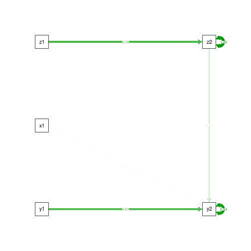
summary(fit.noCtrlT1.yz)
## lavaan (0.5-20) converged normally after  13 iterations
##
##   Number of observations                           250
##
##   Estimator                                         ML
##   Minimum Function Test Statistic                0.000
##   Degrees of freedom                                 0
##   Minimum Function Value               0.0000000000000
##
## Parameter Estimates:
##
##   Information                                 Expected
##   Standard Errors                             Standard
##
## Regressions:
##                    Estimate  Std.Err  Z-value  P(>|z|)
##   y2 ~
##     x1         (c)    0.151    0.074    2.043    0.041
##     z2         (b)    0.279    0.061    4.588    0.000
##   z2 ~
##     x1         (a)    0.210    0.076    2.761    0.006
##
## Variances:
##                    Estimate  Std.Err  Z-value  P(>|z|)
##     y2                1.334    0.119   11.180    0.000
##     z2                1.446    0.129   11.180    0.000
##
## Defined Parameters:
##                    Estimate  Std.Err  Z-value  P(>|z|)
##     ab                0.059    0.025    2.366    0.018
##     total             0.210    0.076    2.761    0.006
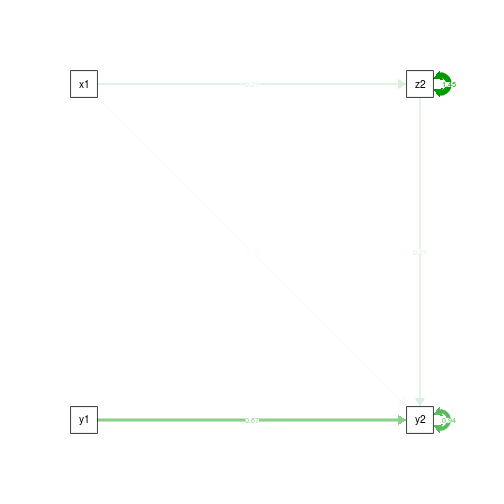
semPaths(fit.noCtrlT1.yz, what='est', rotation=2, exoCov=F, exoVar=F)
You can see that we’re getting a hint that the ab path might be getting bigger as we further misspecify the model. To find out for sure, let’s run the simulations. Our outcome of interest will be the measure of power to detect a significant ab path – the mediated effect. Usually power is a good thing, but if you have power to detect something that’s not there, it’s an indication that your model is reliably giving you the wrong answer.
Again, if you want to redo these simulations, you can set REDOSIMS=T.
REDOSIMS=F
if(REDOSIMS){
    sim.CtrlT1.yz <- simsem::sim(nRep=1000,
                                 model=mediationModelControlzT1,
                                 n=250,
                                 generate=generatingModel,
                                 lavaanfun="sem",
                                 std.lv=F,
                                 multicore=T)
    sim.noCtrlT1.z <- simsem::sim(nRep=1000,
                                  model=mediationModelNoControlzT1,
                                  n=250,
                                  generate=generatingModel,
                                  lavaanfun="sem",
                                  std.lv=F,
                                  multicore=T)
    sim.noCtrlT1.yz <- simsem::sim(nRep=1000,
                                   model=mediationModelNoControlzOryT1,
                                   n=250,
                                   generate=generatingModel,
                                   lavaanfun="sem",
                                   std.lv=F,
                                   multicore=T)
    saveRDS(object=sim.CtrlT1.yz, file='sim_CtrlT1_yz.RDS')
    saveRDS(object=sim.noCtrlT1.z, file='sim_noCtrlT1_z.RDS')
    saveRDS(object=sim.noCtrlT1.yz, file='sim_noCtrlT1_yz.RDS')
} else {
    sim.CtrlT1.yz <- readRDS(file='sim_CtrlT1_yz.RDS')
    sim.noCtrlT1.z <- readRDS(file='sim_noCtrlT1_z.RDS')
    sim.noCtrlT1.yz <- readRDS(file='sim_noCtrlT1_yz.RDS')
}
kable(summaryParam(sim.CtrlT1.yz), digits=2)
| Estimate Average | Estimate SD | Average SE | Power (Not equal 0) | Std Est | Std Est SD | Std Ave SE | |
|---|---|---|---|---|---|---|---|
| y2~y1 | 0.67 | 0.07 | 0.06 | 1.00 | 0.55 | 0.05 | 0.04 |
| c | -0.04 | 0.07 | 0.06 | 0.08 | -0.03 | 0.05 | 0.05 |
| b | 0.21 | 0.05 | 0.05 | 0.98 | 0.21 | 0.05 | 0.05 |
| a | 0.00 | 0.07 | 0.07 | 0.06 | 0.00 | 0.05 | 0.05 |
| z2~z1 | 0.70 | 0.07 | 0.07 | 1.00 | 0.57 | 0.05 | 0.04 |
| y2~~y2 | 0.92 | 0.08 | 0.08 | 1.00 | 0.62 | 0.05 | 0.04 |
| z2~~z2 | 0.99 | 0.09 | 0.09 | 1.00 | 0.67 | 0.05 | 0.04 |
| ab | 0.00 | 0.01 | 0.01 | 0.03 | 0.00 | 0.01 | 0.01 |
| total | -0.04 | 0.07 | 0.07 | 0.09 | -0.03 | 0.06 | 0.05 |
kable(summaryParam(sim.noCtrlT1.z), digits=2)
| Estimate Average | Estimate SD | Average SE | Power (Not equal 0) | Std Est | Std Est SD | Std Ave SE | |
|---|---|---|---|---|---|---|---|
| y2~y1 | 0.67 | 0.07 | 0.06 | 1.00 | 0.56 | 0.05 | 0.04 |
| c | -0.04 | 0.07 | 0.06 | 0.08 | -0.03 | 0.05 | 0.05 |
| b | 0.21 | 0.05 | 0.05 | 0.99 | 0.21 | 0.05 | 0.05 |
| a | 0.21 | 0.08 | 0.08 | 0.78 | 0.17 | 0.06 | 0.06 |
| y2~~y2 | 0.92 | 0.08 | 0.08 | 1.00 | 0.64 | 0.05 | 0.04 |
| z2~~z2 | 1.44 | 0.13 | 0.13 | 1.00 | 0.97 | 0.02 | 0.02 |
| ab | 0.04 | 0.02 | 0.02 | 0.64 | 0.04 | 0.02 | 0.02 |
| total | 0.01 | 0.07 | 0.07 | 0.06 | 0.01 | 0.06 | 0.05 |
kable(summaryParam(sim.noCtrlT1.yz), digits=2)
| Estimate Average | Estimate SD | Average SE | Power (Not equal 0) | Std Est | Std Est SD | Std Ave SE | |
|---|---|---|---|---|---|---|---|
| c | 0.15 | 0.08 | 0.07 | 0.52 | 0.12 | 0.06 | 0.06 |
| b | 0.28 | 0.06 | 0.06 | 1.00 | 0.28 | 0.06 | 0.06 |
| a | 0.21 | 0.08 | 0.08 | 0.78 | 0.17 | 0.06 | 0.06 |
| y2~~y2 | 1.32 | 0.12 | 0.12 | 1.00 | 0.89 | 0.04 | 0.04 |
| z2~~z2 | 1.44 | 0.13 | 0.13 | 1.00 | 0.97 | 0.02 | 0.02 |
| ab | 0.06 | 0.03 | 0.03 | 0.69 | 0.05 | 0.02 | 0.02 |
| total | 0.21 | 0.08 | 0.08 | 0.78 | 0.17 | 0.06 | 0.06 |
Looking across those ab lines, you see that we’re not too bad off if we control for our wave 1 measurements. However, if we don’t do that, we end up with ~64-69% power to detect a significant mediation. To me, this warrants extreme caution.