The RI-CLPM in OpenMx
September 26, 2018
Lavaan is great. I love lavaan. But a lot of folks prefer OpenMx, and given its long and widespread usage, especially in fields outside psychology, it might be a bit better road tested. So this is a brief addendum to my previous post, showing you how to implement a RI-CLPM in OpenMx.
RI-CLPM
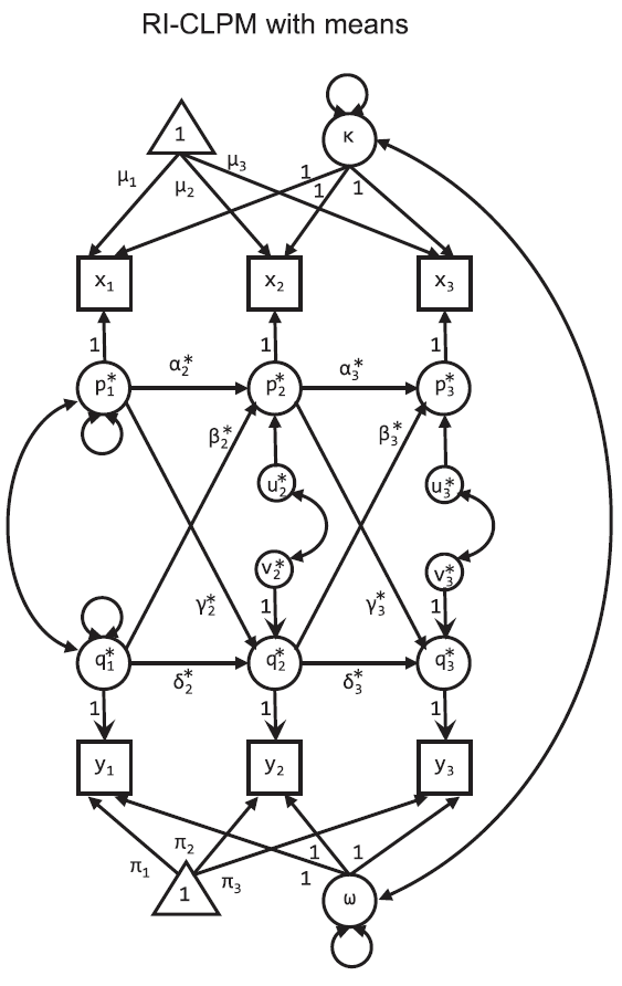
As a reminder, the model looks like this:
The packages
#if you need to install anything, uncomment the below install lines for now
#install.packages('OpenMx')
#install.packages('tidyverse')
require(OpenMx)
require(tidyverse)
Some data: a reminder
I’ll use the same data from before, which was presented on at a methods symposium at SRCD in 1997. Supporting documentation can be found in this pdf. Data and code for importing it was helpfully provided by Sanjay Srivastava.
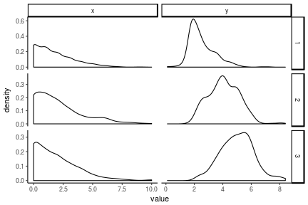
The variables we’re considering are a measure of antisocial behavior (anti) and reading recognition (read). See the docs for descriptions of the other variables. And for the purpose of the model fitting below, x <- anit and y <- read. Following are some descriptions of the raw data:
antiread <- read.table("srcddata.dat",
                       na.strings = c("999.00"),
                       col.names = c("anti1", "anti2", "anti3", "anti4",
                                     "read1", "read2", "read3", "read4",
                                     "gen", "momage", "kidage", "homecog",
                                     "homeemo", "id")
) %>%
  rename(x1 = anti1, x2 = anti2, x3 = anti3, x4 = anti4,
         y1 = read1, y2 = read2, y3 = read3, y4 = read4) %>%
  select(matches('[xy][1-4]'))

knitr::kable(summary(antiread), format = 'markdown')
| x1 | x2 | x3 | x4 | y1 | y2 | y3 | y4 | |
|---|---|---|---|---|---|---|---|---|
| Min. :0.000 | Min. : 0.000 | Min. : 0.000 | Min. : 0.000 | Min. :0.100 | Min. :1.600 | Min. :2.200 | Min. :2.500 | |
| 1st Qu.:0.000 | 1st Qu.: 0.000 | 1st Qu.: 0.000 | 1st Qu.: 0.000 | 1st Qu.:1.800 | 1st Qu.:3.300 | 1st Qu.:4.200 | 1st Qu.:4.925 | |
| Median :1.000 | Median : 1.500 | Median : 1.000 | Median : 1.500 | Median :2.300 | Median :4.100 | Median :5.000 | Median :5.800 | |
| Mean :1.662 | Mean : 2.027 | Mean : 1.828 | Mean : 2.061 | Mean :2.523 | Mean :4.076 | Mean :5.005 | Mean :5.774 | |
| 3rd Qu.:3.000 | 3rd Qu.: 3.000 | 3rd Qu.: 3.000 | 3rd Qu.: 3.000 | 3rd Qu.:3.000 | 3rd Qu.:4.900 | 3rd Qu.:5.800 | 3rd Qu.:6.675 | |
| Max. :9.000 | Max. :10.000 | Max. :10.000 | Max. :10.000 | Max. :7.200 | Max. :8.200 | Max. :8.400 | Max. :8.300 | |
| NA | NA’s :31 | NA’s :108 | NA’s :111 | NA | NA’s :30 | NA’s :130 | NA’s :135 |
antiread %>%
  select(-x4,-y4) %>%
  mutate(pid = 1:n()) %>%
  gather(key, value, -pid) %>%
  extract(col = key, into = c('var', 'wave'), regex = '(\\w)(\\d)') %>%
  ggplot(aes(x = value)) +
  geom_density(alpha = 1) +
  facet_grid(wave~var, scales = 'free') +
  theme_classic()
## Warning: Removed 299 rows containing non-finite values (stat_density).
antireadLong <- antiread %>%
select(-x4,-y4) %>%
mutate(pid = 1:n()) %>%
gather(key, value, -pid) %>%
extract(col = key, into = c('var', 'wave'), regex = '(\\w)(\\d)')
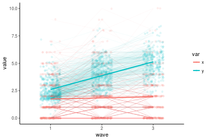
antireadLong %>%
ggplot(aes(x = wave, y = value, color = var, group = var)) +
geom_point(position = position_jitter(w = .2), alpha = .1) +
geom_line(stat = 'identity', aes(group = interaction(var, pid)), alpha = .04) +
geom_line(stat = 'smooth', method = 'lm', size = 1) +
theme_classic()
## Warning: Removed 299 rows containing non-finite values (stat_smooth).
## Warning: Removed 299 rows containing missing values (geom_point).
## Warning: Removed 271 rows containing missing values (geom_path).
Fitting a RI-CLPM in OpenMx
Below is the code to specify and fit the RI-CLPM with equality constraints on the autoregressive, cross-lagged, and residual (for wave 2 and 3) paths (see this in lavaan here).
If you’re not familiar with OpenMx syntax, but you know what a latent growth curve model looks like, check out the OpenMx LGCM example. You construct your model using a series of functions to create each element. Note that OpenMx likes everything to be very explicit, which can be a good thing. You should think about and specify reasonable starting values, and you should be prepared to put bounds on variables that have them (e.g., variances shouldn’t be negative). I’ll call these out as they come up. Also, equality constraints are achieved through the use of path labels, and so I’ll introduce some shorthand to create labels with similar or identical names.
Data specification
antireadRaw <- mxData(observed = antiread, type = 'raw')
This specifies that the data is in the antiread data.frame, with ‘raw’ indicating that it is not a covariance matrix, but rather a data.frame with a row per observation, and a column per variable. It will look in the column names for any manifest variables that are specified.
manifestsX <- c('x1', 'x2', 'x3')
manifestsY <- c('y1', 'y2', 'y3')

latentResX <- c('p1', 'p2', 'p3')
latentResY <- c('q1', 'q2', 'q3')
The above is just to be able to have single variables that contain all the manifest and latent variables I will be using for each construct. Note that these are all the manifests, but not all the latents.
Latent intercepts
kappa <- mxPath(from = "kappa", to = manifestsX,
                arrows = 1, values = c(1,1,1), free = FALSE)
omega <- mxPath(from = "omega", to = manifestsY,
                arrows = 1, values = c(1,1,1), free = FALSE)

print(omega)
## mxPath
## omega -> y1 [value=1, free=FALSE]
## omega -> y2 [value=1, free=FALSE]
## omega -> y3 [value=1, free=FALSE]
This is how to specify the two latent random intercepts. Keep track of the names you use here, because you will need to indicate them in the model construction call. Also, note that printing the resulting variables gives helpful information you can check against your intended specification. The path weights are set to 1 and set to not be freed for estimation.
latentInterceptVars <- mxPath(from = c('kappa', 'omega'), arrows = 2,
                              free = T, connect = 'unique.pairs',
                              labels = c('kappaVar',
                                         'koCovar',
                                         'omegaVar'),
                              values = c(1, 0, 1),
                              lbound = c(0, NA, 0))
This creates free variance and covariance paths between the random intercepts. The ‘unique.pairs’ option will generate a path between each unique combination of the names you use in the “from” parameter. Giving them labels will help you identify them in the output, but are otherwise not strictly necessary. Note that the starting values are set with variances at 1, and the covariance at 0 (because it could be positive or negative), and lower bounds are set on the variance parameters.
Mean structure
meanPathNames <- unlist(lapply(c('mu', 'pi'), paste, 1:3, sep = ''))
Instead of writing out each of the path labels for the means of each manifest variable, I call the above. It’s more characters than just writing it out, but maybe less prone to typos.
intercepts <- mxPath(from = "one", to = c(manifestsX, manifestsY),
                     arrows = 1, free = TRUE,
                     labels = meanPathNames,
                     values = rep(c(1,3), each =3))
The name “one” is reserved to refer to the intercept, and we allow the paths to be estimated freely, labeled with the names created above. It’s probably not necessary to set starting values here, but I glanced at the histograms above and gave it my best guess, just in case.
Latent temporal deviations
latentRes <- mxPath(from = c(latentResX, latentResY),
                    to = c(manifestsX, manifestsY),
                    arrows = 1, free = F,
                    values = rep(1, 6),
                    connect = 'single')
This call creates the paths to the latent variables that are also sometimes called “latent residuals.” Each of the latent variable paths is fixed to 1.
arPaths <- mxPath(from = c(latentResX[1:2], latentResY[1:2]),
                  to = c(latentResX[2:3], latentResY[2:3]),
                  arrows = 1, free = T, connect = 'single',
                  labels = c(rep('alpha', 2), rep('delta', 2)),
                  values = .2)

lagPaths <- mxPath(from = c(latentResX[1:2], latentResY[1:2]),
                  to = c(latentResY[2:3], latentResX[2:3]),
                  arrows = 1, free = T, connect = 'single',
                  labels = c(rep('gamma', 2), rep('beta', 2)),
                  value = 0)

print(arPaths)
## mxPath
## p1 -> p2 [value=0.2, free=TRUE, label='alpha']
## p2 -> p3 [value=0.2, free=TRUE, label='alpha']
## q1 -> q2 [value=0.2, free=TRUE, label='delta']
## q2 -> q3 [value=0.2, free=TRUE, label='delta']
print(lagPaths)
## mxPath
## p1 -> q2 [value=0, free=TRUE, label='gamma']
## p2 -> q3 [value=0, free=TRUE, label='gamma']
## q1 -> p2 [value=0, free=TRUE, label='beta']
## q2 -> p3 [value=0, free=TRUE, label='beta']
These calls establish the paths between the latent residuals. In the first call (that creates the arPaths variable) the first two latent variables for X and Y are connected to the second two. In the second call (that creates the lagPaths variable), the first two X and Y variables are connected to the second two Y and X variables, respectively, to establish the lagged relations. Paths with the same labels are constrained to equality, which is why these paths have the labels assigned as they do. The starting values are based on the expectation that the autoregressive paths are probably positive.
Residual variance structure
resVar <- mxPath(from = c(latentResX, latentResY),
                 arrows = 2, free = T,
                 labels = paste0(c(rep('u',3), rep ('v',3)),
                                 c('1', '', '')),
                 connect = 'single',
                 value = 1, lbound = 0)

resCovar <- mxPath(from = latentResX,
                   to = latentResY,
                   arrows = 2, free = T,
                   labels = paste0(rep ('rescovar',3),
                                   c('1', '', '')),
                   connect = 'single',
                   value = 0)
Finally, the residuals have to be specified. Any path left unspecified will not be included in the model – unlike lavaan, OpenMx doesn’t assume anything about your model. Note that the code paste0(c(rep('u',3), rep ('v',3)), c('1', '', '')) results in the labels: u1, u, u, v1, v, v. These labels constrain the residuals (or disturbances) from wave 2 and 3 to be equal, with those from wave 1 estimated freely. The bivariate covariance is similarly constrained via the labels generated by paste0(rep ('rescovar',3), c('1', '', '')): rescovar1, rescovar, rescovar. Again, the ‘value’ and ‘lbound’ options are set to a reasonable value for the variances. The starting value for the covariances is also set explicitly, though 0 is the default.
Fitting the model and viewing output
riclpm <- mxModel('RICLPM', type = 'RAM',
                  manifestVars = c(manifestsX, manifestsY),
                  latentVars = c(latentResX, latentResY,
                                 'kappa', 'omega'),
                  antireadRaw,
                  kappa,
                  omega,
                  latentInterceptVars,
                  intercepts,
                  latentRes,
                  arPaths,
                  lagPaths,
                  resVar,
                  resCovar)
This call actually puts everything together, translating the path specification into estimable matrices. The first argument is the model name (whatever you wish to call it). After that, you must specify all manifest and latent variables that appear in the path specifications (except for “one”). The rest of the call includes all of the path constructors we generated in the above code (including the data specification).
mxOption(NULL,"Default optimizer","CSOLNP")
riclpm_fit <- mxRun(riclpm)
## Running RICLPM with 19 parameters
This is how you run the model. The optimizer “CSOLNP” is already the default, but I’ve included this code because often convergence issues can be solved by changing the optimizer. Check out the help on the mxOption function for more info. Passing your model variable to the mxRun function is where the magic happens.
summary(riclpm_fit)
## Summary of RICLPM
##
## free parameters:
##         name matrix   row   col    Estimate  Std.Error A lbound ubound
## 1      alpha      A    p2    p1  0.30604054 0.09194632
## 2      gamma      A    q2    p1 -0.03907640 0.03051416
## 3       beta      A    p2    q1 -0.21187505 0.14789152
## 4      delta      A    q2    q1  0.71263799 0.07591069
## 5         u1      S    p1    p1  1.71796121 0.25419453        0
## 6          u      S    p2    p2  2.56920450 0.19932832        0
## 7  rescovar1      S    p1    q1 -0.05643856 0.14585502
## 8         v1      S    q1    q1  0.53528020 0.16608606        0
## 9   rescovar      S    p2    q2 -0.11632638 0.05968509
## 10         v      S    q2    q2  0.59039300 0.03577737        0
## 11  kappaVar      S kappa kappa  1.05159902 0.25302282        0
## 12   koCovar      S kappa omega -0.04570729 0.14256251
## 13  omegaVar      S omega omega  0.32016254 0.16727194        0
## 14       mu1      M     1    x1  1.66172802 0.08269640
## 15       mu2      M     1    x2  1.99042683 0.09980390
## 16       mu3      M     1    x3  1.88963264 0.11131688
## 17       pi1      M     1    y1  2.52271584 0.04595897
## 18       pi2      M     1    y2  4.06661921 0.05511448
## 19       pi3      M     1    y3  5.01826850 0.06430956
##
## Model Statistics:
##                |  Parameters  |  Degrees of Freedom  |  Fit (-2lnL units)
##        Model:             19                   2112              6782.158
##    Saturated:             27                   2104                    NA
## Independence:             12                   2119                    NA
## Number of observations/statistics: 405/2131
##
## Information Criteria:
##       |  df Penalty  |  Parameters Penalty  |  Sample-Size Adjusted
## AIC:       2558.158               6820.158                 6822.132
## BIC:      -5898.052               6896.231                 6835.942
## To get additional fit indices, see help(mxRefModels)
## timestamp: 2018-09-26 17:22:28
## Wall clock time: 0.1292243 secs
## optimizer:  CSOLNP
## OpenMx version number: 2.9.6
## Need help?  See help(mxSummary)
If you compare the fitted model summary to the lavaan output in the previous post, you’ll see they match up very nicely.
Unconstraining and comparing fits
Editing an OpenMx model is fairly straightforward. In order to compare the model with and without equality constraints, we can create new path definitions without the label constraints, then call the mxModel function again with the original model and the new path elements. It will overwrite the old paths with the new specifications.
#free autoregressive and cross-lagged paths
arPaths_uc <- mxPath(
  from = c(latentResX[1:2], latentResY[1:2]),
  to = c(latentResX[2:3], latentResY[2:3]),
  arrows = 1, free = T, connect = 'single',
  labels = paste0(c(rep('alpha', 2), rep('delta', 2)), 1:2),
  values = .2)
lagPaths_uc <- mxPath(
  from = c(latentResX[1:2], latentResY[1:2]),
  to = c(latentResY[2:3], latentResX[2:3]),
  arrows = 1, free = T, connect = 'single',
  labels = paste0(c(rep('gamma', 2), rep('beta', 2)), 1:2),
  value = 0)

#free residuals
resVar_uc <- mxPath(
  from = c(latentResX, latentResY),
  arrows = 2, free = T,
  labels = paste0(c(rep('u',3), rep ('v',3)),
                  1:3),
  connect = 'single',
  value = 1, lbound = 0)

resCovar_uc <- mxPath(
  from = latentResX,
  to = latentResY,
  arrows = 2, free = T,
  labels = paste0(rep ('rescovar',3),
                  1:3),
  connect = 'single',
  value = 0)

riclpm_uc <- mxModel(riclpm,
                     arPaths_uc, lagPaths_uc,
                     resVar_uc, resCovar_uc,
                     name = "RICLPM UC")

summary(riclpm_uc_fit <- mxRun(riclpm_uc))
## Running RICLPM UC with 26 parameters
## Summary of RICLPM UC
##
## free parameters:
##         name matrix   row   col     Estimate  Std.Error A lbound ubound
## 1     alpha1      A    p2    p1  0.162484732 0.16897508
## 2     gamma1      A    q2    p1 -0.057561087 0.07843618
## 3     alpha2      A    p3    p2  0.352612940 0.07752322
## 4     gamma2      A    q3    p2 -0.008105237 0.03363872
## 5      beta1      A    p2    q1 -0.089544921 0.45570009
## 6     delta1      A    q2    q1  0.374146351 0.35005315
## 7      beta2      A    p3    q2 -0.274430873 0.15349585
## 8     delta2      A    q3    q2  0.737837863 0.07340915
## 9         u1      S    p1    p1  1.504287257 0.28044074        0
## 10        u2      S    p2    p2  2.821441372 0.31594765        0
## 11        u3      S    p3    p3  2.109697219 0.20402446        0
## 12 rescovar1      S    p1    q1  0.017013374 0.15930937
## 13        v1      S    q1    q1  0.315640287 0.17213266        0
## 14 rescovar2      S    p2    q2 -0.116941167 0.11390653
## 15        v2      S    q2    q2  0.582452465 0.08547403        0
## 16 rescovar3      S    p3    q3 -0.114698904 0.07061014
## 17        v3      S    q3    q3  0.509168510 0.04576731        0
## 18  kappaVar      S kappa kappa  1.231980754 0.27065286        0
## 19   koCovar      S kappa omega -0.118491763 0.15683489
## 20  omegaVar      S omega omega  0.538749506 0.17694636        0
## 21       mu1      M     1    x1  1.661728759 0.08219595
## 22       mu2      M     1    x2  1.985451719 0.10346911
## 23       mu3      M     1    x3  1.898120810 0.10749165
## 24       pi1      M     1    y1  2.522715853 0.04593036
## 25       pi2      M     1    y2  4.065972155 0.05474760
## 26       pi3      M     1    y3  5.023311788 0.06413183
##
## Model Statistics:
##                |  Parameters  |  Degrees of Freedom  |  Fit (-2lnL units)
##        Model:             26                   2105              6762.106
##    Saturated:             27                   2104                    NA
## Independence:             12                   2119                    NA
## Number of observations/statistics: 405/2131
##
## Information Criteria:
##       |  df Penalty  |  Parameters Penalty  |  Sample-Size Adjusted
## AIC:       2552.106               6814.106                 6817.821
## BIC:      -5876.076               6918.207                 6835.706
## To get additional fit indices, see help(mxRefModels)
## timestamp: 2018-09-26 17:22:28
## Wall clock time: 0.2689583 secs
## optimizer:  CSOLNP
## OpenMx version number: 2.9.6
## Need help?  See help(mxSummary)
The comparison can be made using mxCompare:
mxCompare(riclpm_uc_fit, riclpm_fit)
##        base comparison ep minus2LL   df      AIC   diffLL diffdf
## 1 RICLPM UC       <NA> 26 6762.106 2105 2552.106       NA     NA
## 2 RICLPM UC     RICLPM 19 6782.158 2112 2558.158 20.05131      7
##            p
## 1         NA
## 2 0.00545991
Note that the default output uses the degrees-of-freedom penalized AIC. The conclusion is still the same, though – the constrained model fits more poorly, significantly so if you believe the statistical test.
Here are the estimated parameters:
summary(riclpm_uc_fit)
## Summary of RICLPM UC
##
## free parameters:
##         name matrix   row   col     Estimate  Std.Error A lbound ubound
## 1     alpha1      A    p2    p1  0.162484732 0.16897508
## 2     gamma1      A    q2    p1 -0.057561087 0.07843618
## 3     alpha2      A    p3    p2  0.352612940 0.07752322
## 4     gamma2      A    q3    p2 -0.008105237 0.03363872
## 5      beta1      A    p2    q1 -0.089544921 0.45570009
## 6     delta1      A    q2    q1  0.374146351 0.35005315
## 7      beta2      A    p3    q2 -0.274430873 0.15349585
## 8     delta2      A    q3    q2  0.737837863 0.07340915
## 9         u1      S    p1    p1  1.504287257 0.28044074        0
## 10        u2      S    p2    p2  2.821441372 0.31594765        0
## 11        u3      S    p3    p3  2.109697219 0.20402446        0
## 12 rescovar1      S    p1    q1  0.017013374 0.15930937
## 13        v1      S    q1    q1  0.315640287 0.17213266        0
## 14 rescovar2      S    p2    q2 -0.116941167 0.11390653
## 15        v2      S    q2    q2  0.582452465 0.08547403        0
## 16 rescovar3      S    p3    q3 -0.114698904 0.07061014
## 17        v3      S    q3    q3  0.509168510 0.04576731        0
## 18  kappaVar      S kappa kappa  1.231980754 0.27065286        0
## 19   koCovar      S kappa omega -0.118491763 0.15683489
## 20  omegaVar      S omega omega  0.538749506 0.17694636        0
## 21       mu1      M     1    x1  1.661728759 0.08219595
## 22       mu2      M     1    x2  1.985451719 0.10346911
## 23       mu3      M     1    x3  1.898120810 0.10749165
## 24       pi1      M     1    y1  2.522715853 0.04593036
## 25       pi2      M     1    y2  4.065972155 0.05474760
## 26       pi3      M     1    y3  5.023311788 0.06413183
##
## Model Statistics:
##                |  Parameters  |  Degrees of Freedom  |  Fit (-2lnL units)
##        Model:             26                   2105              6762.106
##    Saturated:             27                   2104                    NA
## Independence:             12                   2119                    NA
## Number of observations/statistics: 405/2131
##
## Information Criteria:
##       |  df Penalty  |  Parameters Penalty  |  Sample-Size Adjusted
## AIC:       2552.106               6814.106                 6817.821
## BIC:      -5876.076               6918.207                 6835.706
## To get additional fit indices, see help(mxRefModels)
## timestamp: 2018-09-26 17:22:28
## Wall clock time: 0.2689583 secs
## optimizer:  CSOLNP
## OpenMx version number: 2.9.6
## Need help?  See help(mxSummary)
You can also request standardized parameters (here, for the constrained model):
mxStandardizeRAMpaths(riclpm_fit, SE = T)
##               name     label matrix   row   col   Raw.Value     Raw.SE
## 1    RICLPM.A[1,7]      <NA>      A    x1    p1  1.00000000 0.00000000
## 2    RICLPM.A[8,7]     alpha      A    p2    p1  0.30604054 0.09194632
## 3   RICLPM.A[11,7]     gamma      A    q2    p1 -0.03907640 0.03051416
## 4    RICLPM.A[2,8]      <NA>      A    x2    p2  1.00000000 0.00000000
## 5    RICLPM.A[9,8]     alpha      A    p3    p2  0.30604054 0.09194632
## 6   RICLPM.A[12,8]     gamma      A    q3    p2 -0.03907640 0.03051416
## 7    RICLPM.A[3,9]      <NA>      A    x3    p3  1.00000000 0.00000000
## 8   RICLPM.A[4,10]      <NA>      A    y1    q1  1.00000000 0.00000000
## 9   RICLPM.A[8,10]      beta      A    p2    q1 -0.21187505 0.14789152
## 10 RICLPM.A[11,10]     delta      A    q2    q1  0.71263799 0.07591069
## 11  RICLPM.A[5,11]      <NA>      A    y2    q2  1.00000000 0.00000000
## 12  RICLPM.A[9,11]      beta      A    p3    q2 -0.21187505 0.14789152
## 13 RICLPM.A[12,11]     delta      A    q3    q2  0.71263799 0.07591069
## 14  RICLPM.A[6,12]      <NA>      A    y3    q3  1.00000000 0.00000000
## 15  RICLPM.A[1,13]      <NA>      A    x1 kappa  1.00000000 0.00000000
## 16  RICLPM.A[2,13]      <NA>      A    x2 kappa  1.00000000 0.00000000
## 17  RICLPM.A[3,13]      <NA>      A    x3 kappa  1.00000000 0.00000000
## 18  RICLPM.A[4,14]      <NA>      A    y1 omega  1.00000000 0.00000000
## 19  RICLPM.A[5,14]      <NA>      A    y2 omega  1.00000000 0.00000000
## 20  RICLPM.A[6,14]      <NA>      A    y3 omega  1.00000000 0.00000000
## 21   RICLPM.S[7,7]        u1      S    p1    p1  1.71796121 0.25419453
## 22  RICLPM.S[10,7] rescovar1      S    q1    p1 -0.05643856 0.14585502
## 23   RICLPM.S[8,8]         u      S    p2    p2  2.56920450 0.19932832
## 24  RICLPM.S[11,8]  rescovar      S    q2    p2 -0.11632638 0.05968509
## 25   RICLPM.S[9,9]         u      S    p3    p3  2.56920450 0.19932832
## 26  RICLPM.S[12,9]  rescovar      S    q3    p3 -0.11632638 0.05968509
## 27 RICLPM.S[10,10]        v1      S    q1    q1  0.53528020 0.16608606
## 28 RICLPM.S[11,11]         v      S    q2    q2  0.59039300 0.03577737
## 29 RICLPM.S[12,12]         v      S    q3    q3  0.59039300 0.03577737
## 30 RICLPM.S[13,13]  kappaVar      S kappa kappa  1.05159902 0.25302282
## 31 RICLPM.S[14,13]   koCovar      S omega kappa -0.04570729 0.14256251
## 32 RICLPM.S[14,14]  omegaVar      S omega omega  0.32016254 0.16727194
##      Std.Value       Std.SE
## 1   0.78759195 5.368619e-02
## 2   0.24138839 7.382613e-02
## 3  -0.05497441 4.382509e-02
## 4   0.85100593 3.707330e-02
## 5   0.29881098 8.684717e-02
## 6  -0.06342326 4.956579e-02
## 7   0.85653817 3.791408e-02
## 8   0.79103394 1.213583e-01
## 9  -0.09328270 6.582846e-02
## 10  0.55962731 9.023985e-02
## 11  0.85471662 7.897057e-02
## 12 -0.11598152 8.120753e-02
## 13  0.64847673 6.643914e-02
## 14  0.87523478 6.957208e-02
## 15  0.61619714 6.861897e-02
## 16  0.52515608 6.007661e-02
## 17  0.51608368 6.292557e-02
## 18  0.61177227 1.569187e-01
## 19  0.51909488 1.300291e-01
## 20  0.48369833 1.258882e-01
## 21  1.00000000 1.463091e-14
## 22 -0.05885436 1.470338e-01
## 23  0.93037949 3.831862e-02
## 24 -0.07513604 3.937617e-02
## 25  0.88694219 5.568539e-02
## 26 -0.06675615 3.462057e-02
## 27  1.00000000 6.625593e-12
## 28  0.68017376 1.045606e-01
## 29  0.56321047 8.684052e-02
## 30  1.00000000 1.582982e-14
## 31 -0.07877259 2.360775e-01
## 32  1.00000000 2.268831e-12
Plotting model expectations
There are just a couple of changes to the code from the previous post having to do with how we extract information from the fitted model.
#get the model-expected means
means <- mxGetExpected(riclpm_fit, component = 'means')
meansDF <- data.frame(mean = means[1,], key = dimnames(means)[[2]]) %>%
  extract(col = key, into = c('var', 'wave'), regex = '(\\w)(\\d)')

factorScores <- mxFactorScores(riclpm_fit, type = 'regression', minManifests = 0)

#plot the model-expected random intercepts
as.data.frame(factorScores[,,1]) %>%
  mutate(pid = 1:n()) %>%
  gather(key, latentvalue, -pid, -kappa, -omega) %>%
  extract(col = key, into = c('latentvar', 'wave'), regex = '(\\w)(\\d)') %>%
  mutate(var = c(p = 'x', q = 'y')[latentvar]) %>%
  left_join(meansDF) %>% #those means from above
  left_join(antireadLong, by = c('pid', 'wave', 'var')) %>% #the raw data
  mutate(expectedLine = ifelse(var == 'x', kappa, omega) + mean,
         wave = as.numeric(wave)) %>%
  rowwise() %>%
  ggplot(aes(x = wave, y = expectedLine, color = var, group = var)) +
  geom_point(aes(x = wave, y = value, group = interaction(var, pid)), alpha = .2, position = position_jitter(w = .2, h = 0)) +
  geom_line(aes(y = expectedLine, group = interaction(var, pid)), stat = 'identity', alpha = .2) +
  geom_line(aes(y = mean), stat = 'identity', alpha = 1, size = 1, color = 'black') +
  facet_wrap(~var, ncol = 2) +
  theme_classic()
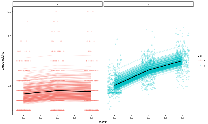
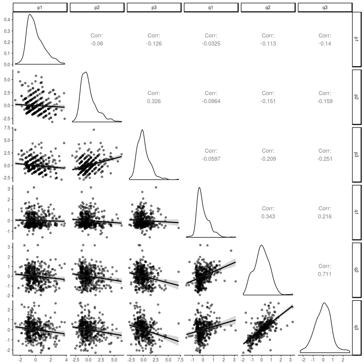
The correlations between the latent residuals from this model are just about as easy to look at as the lavaan version.
library(GGally)
as.data.frame(factorScores[,,1]) %>%
  select(-kappa, -omega) %>%
  ggpairs(lower = list(continuous = wrap(ggally_smooth, alpha = .5))) +
  theme_classic()