Brief MLM tutorial

September 20, 2016

Updated: plotting estimates from real data using predict.

This is a brief description of how to think about multi-level models, especially the link between the formal expression of these models and how that looks in lme4. The data set consists of 4 observations per day over 2 days of cortisol in a developmental sample. The relevant theoretical questions are: what individual-level predictors are related to cortisol intercepts and slopes.

$\begin{equation} \begin{split} \text{cort}_{ij} &=\beta_{0j}+\beta_{1j} \cdot \text{time}_{ij}+\epsilon_{ij}\\ \beta_{0j} &=\gamma_{00}+\gamma_{0[\ldots]}\cdot\text{intercept predictors}+u_{0j}\\ \beta_{1j} &=\gamma_{10}+\gamma_{1[\ldots]}\cdot\text{slope predictors}+u_{1j} \end{split} \label{corteq} \end{equation}$

The model in equation \ref{corteq} says that every ith cortisol observation, for the jth participant, is predicted by an intercept ($\beta_{0j}$), and a linear lope ($\beta_{1j}$). This is equivalent to a linear model that you’re used to in lm: y ~ 1 + time. “$\text{time}_{ij}$”, in this case, is whatever you want to use – it’s probably going to be the time of day the measurement was taken for the ith cortisol observation, for the jth participant.

You’re grouping all your observations by subject, and so you can get a random effect (variation across subjects) for both the intercept and slope. That is, each of those parameters gets its own equation, which you see as the second two parts of eq \ref{corteq}. And just as $\epsilon_{ij}$ is the deviation of every observation from the prediction, $u_{0j}$ and $u_{1j}$ is the deviation of every subject’s predicted intercept and slope from the overall mean intercept and slope across all subjects. It just stands in for the fact that we’re letting the slope and intercept be different for each person.

For $\beta_{0j}$ and $\beta_{1j}$ you might have multiple predictors you’re interested in, so I’ve just indicated that as “$\gamma_{0/1[\ldots]}\cdot\text{intercept/slope predictors}$”. But let’s say you have just one subject level predictor for each of those subject-specific slopes and intercepts. I’ll use SES as the intercept and slope predictor (though you could, in principle, use different predictors for each parameter). The three equations would be:

$\begin{equation} \begin{split} \text{cort}_{ij} &=\beta_{0j}+\beta_{1j} \cdot \text{time}_{ij}+\epsilon_{ij}\\ \beta_{0j} &=\gamma_{00}+\gamma_{01}\cdot\text{SES}_{j}+u_{0j}\\ \beta_{1j} &=\gamma_{10}+\gamma_{11}\cdot\text{SES}_{j}+u_{1j} \end{split} \label{corteqfull} \end{equation}$

When we use lmer to estimate the model, we only give it one equation. So what we need to do is substitute the equations for $\beta_{0j}$ and $\beta_{1j}$ in to get everything in term of the $\gamma$ parameters (notice that our $\text{time}_{ij}$ variable gets multiplied through the equation for $\beta_{1j}$ and creates the interaction term $\text{SES}_{j}\times \text{time}$):

$\begin{equation} \begin{split} \text{cort}_{ij} =& \gamma_{00}+\gamma_{01}\cdot\text{SES}_{j}+u_{0j}+\\ &(\gamma_{10}+\gamma_{11}\cdot\text{SES}_{j}+u_{1j}) \cdot \text{time}_{ij}+\epsilon_{ij}\\ \text{cort}_{ij} =& \gamma_{00}+\gamma_{01}\cdot\text{SES}_{j}+u_{0j}+\\ &\gamma_{10}\cdot \text{time}_{ij}+\gamma_{11}\cdot\text{SES}_{j}\times \text{time}_{ij}+u_{1j}\cdot \text{time}_{ij} +\epsilon_{ij}\\ \text{cort}_{ij} =& \gamma_{00}+\gamma_{01}\cdot\text{SES}_{j}+\gamma_{10}\cdot \text{time}_{ij}+\gamma_{11}\cdot\text{SES}_{j}\times \text{time}_{ij}+\\ &u_{0j}+u_{1j}\cdot \text{time}_{ij} +\epsilon_{ij} \end{split} \label{corteqsingle} \end{equation}$

The final equation in \ref{corteqsingle} is just reordered so that we group our fixed effects together, and our random effects and error together. Also, I’m just using “$\cdot$” and “$\times$” to set apart parameters and variable interactions a bit.

So now we have our full model equation, and we can give it to lmer:

aModel <- lmer(cort ~ 1 + SES + time + SES:time + 
                     (1 + time | SID), 
               data=yourData)
summary(aModel)

It doesn’t really matter that you have two days of data per person, because we just care about the time of day. You could potentially add another grouping by day, but it might make things more complicated than necessary.

When you get output from summary, you’ll look at the term SES:time to see if a subject’s SES predicts their cortisol slope. This is because in equation \ref{corteqfull}, $\gamma_{11}$ is the parameter for SES predicting $\beta_{1j}$, which is your cortisol slope parameter. This parameter sticks around in the final equation \ref{corteqsingle} for the interaction term.

Plotting model estimates

Let’s consider a model and some real data:

lmer(cort ~ 1 + time*ageyrs*SUBTYPE + gender  +steroid + meds +
            (1 | IDENT_SUBID:index4) + (1 + time | IDENT_SUBID),
     data=aDF)

which expands to (grouping terms by the observation-level parameter they seek to explain):

lmer(cort ~ 1 + ageyrs + SUBTYPE + ageyrs:SUBTYPE + gender + steroid + meds +
            time + time:ageyrs + time:SUBTYPE + time:ageyrs:SUBTYPE +
            (1 | IDENT_SUBID:index4) + (1 + time | IDENT_SUBID),
     data=aDF)

aDF <- read.csv('./cort_mini.csv')
head(aDF)

##   IDENT_SUBID SUBTYPE ageyrs gender  time  cort Index1 index4 Indexday
## 1       SB001       0    9.5      0 20.00  1.87      8      4        2
## 2       SB001       0    9.5      0 17.00  1.47      3      3        1
## 3       SB001       0    9.5      0 20.00  0.85      4      4        1
## 4       SB001       0    9.5      0  7.75 13.28      6      2        2
## 5       SB001       0    9.5      0  7.75 11.66      2      2        1
## 6       SB001       0    9.5      0  7.00 11.27      5      1        2
##   sick meds steroid
## 1    0    0       0
## 2    0    0       0
## 3    0    0       0
## 4    0    0       0
## 5    0    0       0
## 6    0    0       0

We have cortisol measured at 4 different times per day (index4), over two days, nested within subjects. As I understand it, grouping by measurement within subject helps account for the possibility that some subjects wake up later than others, and so the intercept of the cortisol measurements for each timepoint may deviate from the expected value.

We have an observation-level variable: time; and several subject-level variables: ageyrs, subtype, gender, steroid, and meds. I think that this lmer call implies the following equations (but I don’t often work with this kind of nesting), where i is the observation index, j is the measurement-within-subject index (IDENT_SUBID:index4), and k is the subject index (IDENT_SUBID):

$\begin{equation} \begin{split} \text{cort}_{ij} = &\beta_{0jk}+\beta_{1jk} \cdot \text{time}_{ij}+\epsilon_{ijk}\\ \beta_{0jk} = &\gamma_{00k}+u_{0jk}\\ \beta_{1jk} = &\gamma_{10k}\\ \gamma_{00k} = &\delta_{000}+\delta_{001} \cdot \text{ageyrs}+\delta_{002} \cdot \text{SUBTYPE}+\delta_{003} \cdot \text{ageyrs:SUBTYPE}+\\ & \delta_{004} \cdot \text{gender}+\delta_{005} \cdot \text{steroid}+\delta_{006} \cdot \text{meds}+v_{00k}\\ \gamma_{10k} = &\delta_{100}+\delta_{101} \cdot \text{ageyrs}+\delta_{102} \cdot \text{SUBTYPE}+\delta_{103} \cdot \text{ageyrs:SUBTYPE}+v_{10k}\\ \end{split} \label{realcorteq} \end{equation}$

We’ll estimate the paramters for this model using the restricted data set in aDF (this is not public data, so we just have a subset of participants).

library(lme4)

## Loading required package: Matrix

aMod <- lmer(cort ~ 1 + ageyrs + SUBTYPE + ageyrs:SUBTYPE + gender + steroid + meds +
            time + time:ageyrs + time:SUBTYPE + time:ageyrs:SUBTYPE +
            (1 | IDENT_SUBID:index4) + (1 + time | IDENT_SUBID),
     data=aDF)
summary(aMod)

## Linear mixed model fit by REML ['lmerMod']
## Formula: 
## cort ~ 1 + ageyrs + SUBTYPE + ageyrs:SUBTYPE + gender + steroid +  
##     meds + time + time:ageyrs + time:SUBTYPE + time:ageyrs:SUBTYPE +  
##     (1 | IDENT_SUBID:index4) + (1 + time | IDENT_SUBID)
##    Data: aDF
## 
## REML criterion at convergence: 1460.6
## 
## Scaled residuals: 
##     Min      1Q  Median      3Q     Max 
## -2.8222 -0.4268 -0.0796  0.4116  4.1111 
## 
## Random effects:
##  Groups             Name        Variance Std.Dev. Corr 
##  IDENT_SUBID:index4 (Intercept)  0.9080  0.9529        
##  IDENT_SUBID        (Intercept) 83.4431  9.1347        
##                     time         0.1799  0.4242   -1.00
##  Residual                       26.2967  5.1280        
## Number of obs: 230, groups:  IDENT_SUBID:index4, 121; IDENT_SUBID, 31
## 
## Fixed effects:
##                       Estimate Std. Error t value
## (Intercept)          22.657372   5.315795   4.262
## ageyrs                0.210303   0.543330   0.387
## SUBTYPE             -10.062975   9.042737  -1.113
## gender                1.828639   1.187347   1.540
## steroid               0.399612   2.209404   0.181
## meds                 -3.987401   3.796144  -1.050
## time                 -1.110025   0.278735  -3.982
## ageyrs:SUBTYPE        1.334753   0.945475   1.412
## ageyrs:time          -0.006866   0.028338  -0.242
## SUBTYPE:time          0.445148   0.473223   0.941
## ageyrs:SUBTYPE:time  -0.048506   0.049015  -0.990
## 
## Correlation of Fixed Effects:
##             (Intr) ageyrs SUBTYPE gender sterod meds   time   ag:SUBTYPE
## ageyrs      -0.901                                                      
## SUBTYPE     -0.585  0.534                                               
## gender      -0.057 -0.067 -0.027                                        
## steroid      0.031 -0.104 -0.044   0.392                                
## meds         0.017 -0.020  0.072  -0.026  0.231                         
## time        -0.955  0.865  0.562  -0.005 -0.011 -0.003                  
## agy:SUBTYPE  0.516 -0.566 -0.888  -0.002 -0.017 -0.145 -0.496           
## ageyrs:time  0.870 -0.954 -0.511   0.002  0.017  0.004 -0.909  0.547    
## SUBTYPE:tim  0.561 -0.510 -0.954   0.013  0.002 -0.007 -0.589  0.843    
## ag:SUBTYPE: -0.502  0.552  0.851  -0.006 -0.008  0.002  0.525 -0.948    
##             agyrs: SUBTYPE:
## ageyrs                     
## SUBTYPE                    
## gender                     
## steroid                    
## meds                       
## time                       
## agy:SUBTYPE                
## ageyrs:time                
## SUBTYPE:tim  0.535         
## ag:SUBTYPE: -0.578 -0.890

The model object in aMod contains enough information that we can create a new data set and use predict to get expected values for plotting the interactions we’re interested in. We’d like to plot the cortisol slope (x = time, y = cort) for different ages (grouping lines by integer ages, say), and we probably want a different plot for each subtype. We also need a value for every term in the model, so let’s get the mean for our “control” variables:

mean_gender = .5 #gender is coded 1 and 0
mean_steroid = .5 #steroid is coded 1 and 0
mean_meds = .5 #ditto

We now want to get all combinations of age (say, every second integer between 4 and 18), subtype (0 and 1), and continuous time (5am - 11pm). We can use expand.grid to do this handily:

predData <- data.frame(expand.grid(ageyrs = seq(4, 18, 2),
                                   SUBTYPE = c(0, 1),
                                   time = seq(5.0, 23.0, .5),
                                   gender = mean_gender,
                                   steroid = mean_steroid,
                                   meds = mean_meds))
head(predData)

##   ageyrs SUBTYPE time gender steroid meds
## 1      4       0    5    0.5     0.5  0.5
## 2      6       0    5    0.5     0.5  0.5
## 3      8       0    5    0.5     0.5  0.5
## 4     10       0    5    0.5     0.5  0.5
## 5     12       0    5    0.5     0.5  0.5
## 6     14       0    5    0.5     0.5  0.5

Now we can call predict to get values for cort (read ?predict.merMod for more info). We’ll set re.form = NA so that it only estimates the fixed effects. We could get expected values of cort for each of our participants, which is fun, but I’ll save that for later.

predData$cort <- predict(object=aMod, newdata=predData, re.form=NA)
head(predData)

##   ageyrs SUBTYPE time gender steroid meds     cort
## 1      4       0    5    0.5     0.5  0.5 16.93157
## 2      6       0    5    0.5     0.5  0.5 17.28352
## 3      8       0    5    0.5     0.5  0.5 17.63547
## 4     10       0    5    0.5     0.5  0.5 17.98742
## 5     12       0    5    0.5     0.5  0.5 18.33937
## 6     14       0    5    0.5     0.5  0.5 18.69132

Now, to plot it using ggplot in the form I hinted at above:

library(ggplot2)
ggplot(predData, aes(x=time, y=cort, group=ageyrs, color=ageyrs))+
       geom_line()+
       facet_wrap(~SUBTYPE)

center

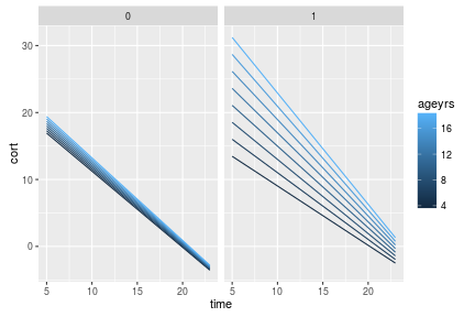
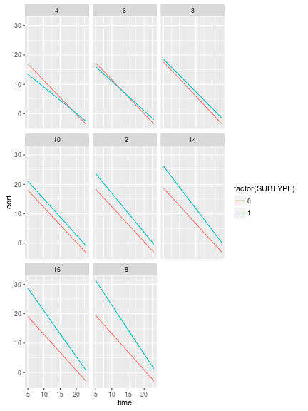
In the plot above you see an interaction with age for SUBTYPE 1, only. There are some other ways to play with this plot, like faceting by age, or letting the color be dictated by an interaction between the two:

library(ggplot2)
ggplot(predData, aes(x=time, y=cort, group=factor(SUBTYPE), color=factor(SUBTYPE)))+
       geom_line()+
       facet_wrap(~ageyrs)

center

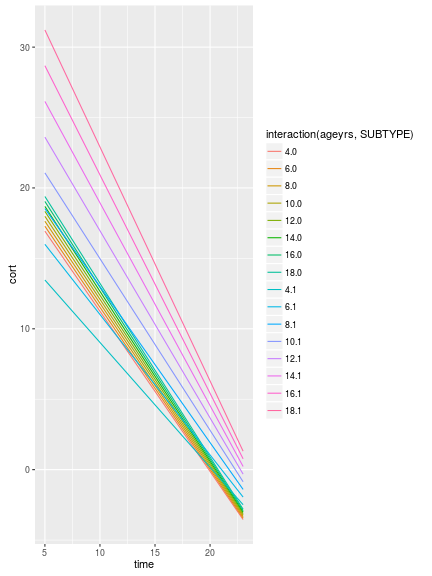
library(ggplot2)
ggplot(predData, aes(x=time, y=cort, group=interaction(ageyrs, SUBTYPE), color=interaction(ageyrs, SUBTYPE)))+
       geom_line()

center