Flow Routing and Accumulation Guide

Last updated: 2026-02-09

This guide documents our learnings from developing and debugging the hydrological flow routing system in terrain-maker. It covers algorithm design, implementation details, debugging strategies, and lessons learned.

Overview

Hydrological flow routing determines how water moves across a terrain surface. The system computes:

• Flow direction: Which neighboring cell each cell drains to (D8 algorithm)

• Drainage area: How many upstream cells contribute flow to each cell

• Upstream rainfall: Precipitation-weighted flow accumulation

---

Part 1: Algorithm Foundations

The Core Problem

Given a Digital Elevation Model (DEM), we want to answer: “If a drop of water falls on cell (i,j), where does it go?”

This seems simple - water flows downhill - but complications arise:

1. Depressions (pits): Natural and artificial sinks where water pools

2. Flat areas: Zero-slope regions with no obvious flow direction

3. NoData boundaries: Ocean, lakes, domain edges

4. Numerical precision: Floating-point artifacts create false gradients

Why D8?

D8 (8-direction) flow assigns each cell exactly one of 8 possible flow directions (or no flow for sinks). Alternatives exist:

Algorithm	Description	Trade-offs
D8	Single steepest descent neighbor	Simple, fast, but can create parallel flow on hillslopes
D-infinity	Proportional flow based on slope angle	More realistic divergence, but complex accumulation
MFD	Multiple flow directions weighted by slope	Best for diffuse flow, expensive to compute

We chose D8 because:

• Simpler accumulation (topological sort works directly)

• Sufficient for stream network extraction

• Standard in GIS tools (ESRI, GRASS, QGIS)

• Easier to debug and validate

The Four-Stage Pipeline

Our implementation follows a spec-compliant pipeline based on peer-reviewed literature:

┌─────────────────────────────────────────────────────────────────┐
│                    STAGE 1: OUTLET IDENTIFICATION               │
│  Classify cells that serve as drainage termini                  │
│  (coastal, edge, masked basin outlets)                          │
└─────────────────────────────────────────────────────────────────┘
                              │
                              ▼
┌─────────────────────────────────────────────────────────────────┐
│               STAGE 2a: CONSTRAINED BREACHING                   │
│  Carve least-cost paths from sinks to outlets                   │
│  Subject to max_breach_depth and max_breach_length              │
│  Algorithm: Dijkstra shortest path (Lindsay 2016)               │
└─────────────────────────────────────────────────────────────────┘
                              │
                              ▼
┌─────────────────────────────────────────────────────────────────┐
│                STAGE 2b: RESIDUAL FILL                          │
│  Priority-flood fill remaining sinks with epsilon gradient      │
│  Algorithm: Barnes et al. (2014)                                │
└─────────────────────────────────────────────────────────────────┘
                              │
                              ▼
┌─────────────────────────────────────────────────────────────────┐
│                 STAGE 3: D8 FLOW DIRECTION                      │
│  Assign steepest descent direction to each cell                 │
│  Every non-sink cell now has exactly one lower neighbor         │
└─────────────────────────────────────────────────────────────────┘
                              │
                              ▼
┌─────────────────────────────────────────────────────────────────┐
│                 STAGE 4: FLOW ACCUMULATION                      │
│  Count upstream contributing cells via topological sort         │
│  Kahn's algorithm ensures correct dependency order              │
└─────────────────────────────────────────────────────────────────┘

---

Part 2: Stage 1 - Outlet Identification

The Key Insight

Before any conditioning, we must know WHERE water can exit the domain. This seems obvious but has subtleties:

Wrong approach: “Just let water flow off edges”

• Creates artificial endorheic basins if interior cells are lower than edges

• Produces inconsistent results depending on domain boundary placement

Right approach: Explicitly classify outlets FIRST, then condition terrain to drain to them.

Outlet Types

Type	Description	Detection	Example
Coastal	Adjacent to ocean/NoData, below threshold	elev < coastal_elev_threshold AND adjacent_to_nodata	River mouths
Edge	On grid boundary	Configurable strategy	Domain boundaries
Masked Basin	Adjacent to pre-masked interior NoData	User-supplied masks	Lakes, endorheic basins

Edge Mode Strategies

The edge_mode parameter controls how boundary cells become outlets:

# All boundary cells are outlets (safest, prevents artificial basins)
edge_mode = "all"

# Only boundary cells that are local minima along the edge
edge_mode = "local_minima"

# Cells where interior neighbors slope toward the edge
edge_mode = "outward_slope"

# No edge outlets (for islands surrounded by ocean)
edge_mode = "none"

What we learned: edge_mode="all" is the safest default. The cost is some edge fragmentation, but this is far preferable to creating artificial closed basins that trap water.

Implementation Pattern: Neighbor Iteration

A pattern we use throughout the codebase for 8-connected neighbors:

# D8 direction codes (ESRI convention) and offsets
D8_CODES = [1, 2, 4, 8, 16, 32, 64, 128]
D8_OFFSETS = [
    (0, 1),   # 1: East
    (-1, 1),  # 2: NE
    (-1, 0),  # 4: North
    (-1, -1), # 8: NW
    (0, -1),  # 16: West
    (1, -1),  # 32: SW
    (1, 0),   # 64: South
    (1, 1),   # 128: SE
]

# Iterate neighbors
for code, (dr, dc) in zip(D8_CODES, D8_OFFSETS):
    nr, nc = r + dr, c + dc
    if 0 <= nr < rows and 0 <= nc < cols:
        # Process neighbor
        pass

Why ESRI codes? Compatibility with ArcGIS, QGIS, and other GIS tools. The power-of-2 encoding also allows bitwise operations for multi-flow algorithms.

---

Part 3: Stage 2a - Constrained Breaching

The Problem with Simple Filling

Traditional depression filling raises ALL sink cells to their spill point elevation. This:

1. Destroys terrain detail: Small valleys become plateaus

2. Creates large flat areas: Problematic for flow direction

3. Doesn’t distinguish real vs. artificial sinks: Sensor noise treated same as Death Valley

Lindsay’s Constrained Breaching

The insight: Instead of raising sinks, LOWER the barriers. Carve narrow channels through ridges to drain depressions.

Key parameters:

Parameter	Meaning	Too Low	Too High
max_breach_depth	Max elevation cut per cell	Many sinks survive to fill	Cuts through real ridges
max_breach_length	Max path length in cells	Long sinks can’t breach	Cuts across wide barriers

Algorithm: Dijkstra Least-Cost Path

For each sink, find the cheapest path to a draining cell:

DIJKSTRA_BREACH(sink_cell, max_depth, max_length):

    # Priority queue: (cost, path_length, row, col)
    PQ = MinHeap()
    PQ.push((0, 0, sink_r, sink_c))

    visited = {}
    parent = {}
    sink_elev = DEM[sink_r, sink_c]

    while PQ not empty:
        cost, length, r, c = PQ.pop()

        if (r, c) in visited:
            continue
        visited[(r, c)] = cost

        # Termination: reached a cell that drains
        if resolved[r, c] and DEM[r, c] <= sink_elev:
            return reconstruct_path(parent, sink, (r, c))

        if outlet[r, c]:
            return reconstruct_path(parent, sink, (r, c))

        # Don't expand beyond max_length
        if length >= max_length:
            continue

        for each neighbor (nr, nc):
            if (nr, nc) in visited or nodata[nr, nc]:
                continue

            # Cost = how much we'd have to cut this cell
            breach_depth = max(0, DEM[nr, nc] - sink_elev)

            if breach_depth > max_depth:
                continue  # Would exceed constraint

            new_cost = cost + breach_depth
            PQ.push((new_cost, length + 1, nr, nc))
            parent[(nr, nc)] = (r, c)

    return None  # No valid breach path

Critical Insight: Cost Metric

The cost metric determines breach behavior:

Cost =	Behavior	Good For
max(0, elev - sink_elev)	Minimize total material removed	General use
1 (constant)	Find shortest path	Noisy DEMs
elev - sink_elev (can be negative)	Find steepest descent	Preserving slopes

We use total material removed because it finds the path that disturbs terrain the least.

Applying the Breach

Once we have a path, we carve it with monotonically decreasing elevation:

def apply_breach(dem, path, epsilon):
    # Work backward from drain point to sink
    # Ensure each cell is lower than the previous

    n = len(path)
    base_elev = dem[path[-1]]  # Drain point elevation

    for i in range(n - 2, -1, -1):  # Reverse order
        r, c = path[i]
        required_elev = base_elev + epsilon * (n - 1 - i)

        # Only lower, never raise
        if dem[r, c] > required_elev:
            dem[r, c] = required_elev

Why epsilon gradient? Ensures the carved channel has consistent downward slope, preventing flat spots that confuse D8.

---

Part 4: Stage 2b - Priority-Flood Fill

Barnes (2014) Algorithm

For sinks that couldn’t be breached, fill them minimally:

PRIORITY_FLOOD_FILL(dem, outlets, epsilon):

    PQ = MinHeap()
    in_queue = array of False

    # Seed with all outlets
    for each outlet (r, c):
        PQ.push((dem[r, c], r, c))
        in_queue[r, c] = True

    while PQ not empty:
        elev, r, c = PQ.pop()

        for each neighbor (nr, nc):
            if in_queue[nr, nc] or nodata[nr, nc]:
                continue

            in_queue[nr, nc] = True

            # If neighbor is lower, raise it
            if dem[nr, nc] < elev + epsilon:
                dem[nr, nc] = elev + epsilon

            PQ.push((dem[nr, nc], nr, nc))

Why Priority Queue?

The priority queue ensures we process cells in order of ascending elevation. This guarantees:

1. When we visit a cell, all lower cells are already resolved

2. Fill happens from outlet inward, naturally creating drainage gradient

3. No cell is visited more than once

The Epsilon Gradient

The epsilon parameter deserves special attention:

Epsilon Value	Effect
Too small (< 1e-6)	Float precision errors create ties/reversals
Too large (> 1e-2)	Distorts elevations in large filled areas
Sweet spot (~1e-4)	Clear gradient without distortion

Rule of thumb: epsilon = 1e-5 * cell_resolution

For a 30m DEM: epsilon = 3e-4 For a 10m DEM: epsilon = 1e-4

---

Part 5: Stage 3 - D8 Flow Direction

After Conditioning

Post-conditioning, every land cell (except outlets) has at least one lower neighbor. D8 is now straightforward:

def compute_d8_flow_direction(dem, nodata, outlets):
    rows, cols = dem.shape
    flow_dir = np.zeros((rows, cols), dtype=np.uint8)

    for r in range(rows):
        for c in range(cols):
            if nodata[r, c]:
                flow_dir[r, c] = 0
                continue

            if outlets[r, c]:
                flow_dir[r, c] = 0  # Terminal
                continue

            # Find steepest descent
            max_slope = -np.inf
            best_dir = 0

            for code, (dr, dc) in zip(D8_CODES, D8_OFFSETS):
                nr, nc = r + dr, c + dc

                if not in_bounds(nr, nc) or nodata[nr, nc]:
                    continue

                dist = np.sqrt(dr*dr + dc*dc)  # 1.0 or sqrt(2)
                slope = (dem[r, c] - dem[nr, nc]) / dist

                if slope > max_slope:
                    max_slope = slope
                    best_dir = code

            flow_dir[r, c] = best_dir

    return flow_dir

Diagonal Distance Matters

A subtle but important detail: diagonal neighbors are further away (sqrt(2) vs 1.0). We must compute slope, not just elevation difference:

# WRONG: Biases toward diagonals
score = dem[r, c] - dem[nr, nc]

# RIGHT: Accounts for distance
dist = 1.0 if dr == 0 or dc == 0 else 1.414
slope = (dem[r, c] - dem[nr, nc]) / dist

Handling Ties

When multiple neighbors have equal steepest slope, we need a tie-breaker. Options:

1. Prefer cardinal directions: N/S/E/W over diagonals

2. Prefer lower elevation: Among equal slopes, pick lower neighbor

3. Random: Adds variety but reduces reproducibility

4. Deterministic priority: Fixed order (e.g., E, NE, N, NW, W, SW, S, SE)

We use deterministic priority for reproducibility.

---

Part 6: Stage 4 - Flow Accumulation

The Dependency Problem

Flow accumulation has a dependency: to know how much water reaches cell A, we must first know how much water reaches all cells that drain INTO A.

This is a topological sort problem.

Kahn’s Algorithm

def compute_flow_accumulation(flow_dir, nodata):
    rows, cols = flow_dir.shape

    # Initialize: each cell contributes 1 (itself)
    flow_acc = np.ones((rows, cols), dtype=np.int64)
    flow_acc[nodata] = 0

    # Compute in-degree (number of upstream cells)
    in_degree = np.zeros((rows, cols), dtype=np.int32)

    for r in range(rows):
        for c in range(cols):
            if flow_dir[r, c] == 0:
                continue

            nr, nc = downstream_cell(r, c, flow_dir[r, c])
            if not nodata[nr, nc]:
                in_degree[nr, nc] += 1

    # Seed queue with cells that have no upstream (headwaters)
    queue = deque()
    for r in range(rows):
        for c in range(cols):
            if not nodata[r, c] and in_degree[r, c] == 0:
                queue.append((r, c))

    cells_processed = 0

    while queue:
        r, c = queue.popleft()
        cells_processed += 1

        d = flow_dir[r, c]
        if d == 0:
            continue  # Outlet or nodata

        nr, nc = downstream_cell(r, c, d)
        if not nodata[nr, nc]:
            # Pass accumulation downstream
            flow_acc[nr, nc] += flow_acc[r, c]

            in_degree[nr, nc] -= 1
            if in_degree[nr, nc] == 0:
                queue.append((nr, nc))

    # Cycle detection
    total_land = np.sum(~nodata)
    if cells_processed != total_land:
        raise ValueError(f"Cycle detected! Processed {cells_processed}/{total_land}")

    return flow_acc

Why This Works

1. Headwaters first: Cells with in_degree=0 have no upstream contributors

2. Propagation: As we process cells, their downstream neighbors’ in-degrees decrease

3. Termination: When a cell’s in-degree hits 0, all its upstream is computed

4. Cycle detection: If we can’t reach all cells, there’s a cycle (conditioning bug)

Weighted Accumulation

For rainfall-weighted accumulation, initialize with precipitation instead of 1:

# Instead of:
flow_acc = np.ones((rows, cols))

# Use:
flow_acc = precipitation.copy()

Everything else stays the same - the topological sort handles it.

---

Part 7: Flat Resolution

The Flat Area Problem

After filling, large flat areas have zero slope. D8 can’t determine flow direction.

Consider a 100x100 cell lake bed at exactly 500.0m elevation. Which way does water flow?

Garbrecht-Martz (1997) Dual-Gradient Solution

The insight: Use TWO gradients combined:

1. Toward gradient: Distance from pour points (water flows toward outlets)

2. Away gradient: Distance from high points (water flows from ridges)

FLAT_RESOLUTION(dem, flat_mask, pour_points, high_points):

    # Gradient 1: Distance from pour points (lower terrain)
    toward_dist = BFS_DISTANCE(flat_mask, pour_points)

    # Gradient 2: Distance from high points (higher terrain)
    away_dist = BFS_DISTANCE(flat_mask, high_points)

    # Combined: Garbrecht-Martz formula
    for each flat cell (r, c):
        increment = epsilon * (toward_dist[r, c] + away_dist[r, c])
        dem[r, c] += increment

Why Both Gradients?

Gradient	Creates Flow Pattern
Toward only	Radial flow to outlet (unrealistic)
Away only	Radial flow from ridges (unrealistic)
Combined	Natural dendritic drainage

Visual Comparison

TOWARD ONLY:           AWAY ONLY:            COMBINED:
    ↓ ↓ ↓                 ↑ ↑ ↑                ↘ ↓ ↙
    → O ←                 → · ←                → O ←
    ↑ ↑ ↑                 ↓ ↓ ↓                ↗ ↑ ↖

(O = outlet)           (· = high point)      (natural drainage)

Implementation Detail: Finding High Points

A “high point” on a flat is a flat cell adjacent to HIGHER terrain:

def find_high_points(dem, flat_mask):
    high_points = np.zeros_like(flat_mask)

    for r, c in flat_cells:
        for nr, nc in neighbors(r, c):
            if dem[nr, nc] > dem[r, c]:
                high_points[r, c] = True
                break

    return high_points

---

Part 8: Water Body Integration

Why Lakes Are Hard

Lakes break the fundamental D8 assumption that water flows to the lowest neighbor:

1. Flat surface: Lake surfaces have zero slope (or tiny wind-driven slopes)

2. Single outlet: All water exits through one pour point

3. Multiple inlets: Streams enter from various points around perimeter

4. Internal routing: Water must traverse the lake interior

Our Solution: BFS Routing

For each lake, use breadth-first search from the outlet to assign flow directions:

def create_lake_routing(lake_mask, outlet_mask, dem):
    flow_dir = np.zeros_like(lake_mask, dtype=np.uint8)

    for lake_id in unique_lakes:
        this_lake = (lake_mask == lake_id)
        outlet = outlet_mask & this_lake

        if not np.any(outlet):
            # Endorheic lake - no outlet
            flow_dir[this_lake] = 0
            continue

        # BFS from outlet
        visited = np.zeros_like(this_lake, dtype=bool)
        queue = deque()

        # Initialize with outlet
        for r, c in outlet_cells:
            visited[r, c] = True
            flow_dir[r, c] = 0  # Outlet is terminal
            queue.append((r, c))

        while queue:
            r, c = queue.popleft()

            for code, (dr, dc) in zip(D8_CODES, D8_OFFSETS):
                nr, nc = r + dr, c + dc

                if this_lake[nr, nc] and not visited[nr, nc]:
                    visited[nr, nc] = True
                    # Flow toward the cell we came from
                    flow_dir[nr, nc] = REVERSE_DIR[code]
                    queue.append((nr, nc))

    return flow_dir

Key Insight: Lakes Have Context

Lakes outside endorheic basins act as CONDUITS:

• Water enters through inlets

• Flows through lake interior

• Exits through outlet

• Continues downstream

Lakes inside endorheic basins act as SINKS:

• Water enters and accumulates

• No outlet to the ocean

• Example: Salton Sea, Great Salt Lake

This distinction is critical and we got it wrong initially.

Inlet Detection

Inlets are cells adjacent to lakes where terrain drains INTO the lake:

def identify_inlets(lake_mask, dem, outlet_mask):
    inlets = {}

    for lake_id in unique_lakes:
        this_lake = (lake_mask == lake_id)
        lake_inlet_cells = []

        # Find cells just outside the lake
        perimeter = dilate(this_lake) & ~this_lake

        for r, c in perimeter_cells:
            # Check if terrain slopes into lake
            for nr, nc in neighbors(r, c):
                if this_lake[nr, nc] and not outlet_mask[nr, nc]:
                    if dem[r, c] > dem[nr, nc]:
                        lake_inlet_cells.append((r, c))
                        break

        inlets[lake_id] = lake_inlet_cells

    return inlets

---

Part 9: Endorheic Basin Handling

What Are Endorheic Basins?

Closed drainage systems with no outlet to the ocean:

• Great Salt Lake (Utah)

• Salton Sea (California)

• Death Valley (California)

• Lake Chad (Africa)

• Caspian Sea (Asia)

• Aral Sea (Asia)

These are REAL features, not artifacts. We must preserve them.

Detection Algorithm

def detect_endorheic_basins(dem, min_size, min_depth, exclude_mask):
    """
    Find closed basins by:
    1. Identify all local minima (sinks)
    2. Grow catchment areas
    3. Filter by size and depth
    """

    # Find local minima
    sinks = find_local_minima(dem, exclude_mask)

    basins = {}
    basin_mask = np.zeros_like(dem, dtype=bool)

    for sink_id, (sink_r, sink_c) in enumerate(sinks):
        # Grow catchment (all cells that drain to this sink)
        catchment = grow_catchment(dem, sink_r, sink_c)

        # Calculate basin metrics
        size = np.sum(catchment)
        depth = compute_fill_depth(dem, catchment)

        # Filter
        if size >= min_size and depth >= min_depth:
            basins[sink_id] = {
                'center': (sink_r, sink_c),
                'size': size,
                'depth': depth,
            }
            basin_mask |= catchment

    return basin_mask, basins

Preservation Strategies

Two independent mechanisms:

Strategy	Parameter	Logic
Size-based	min_basin_size	Large basins are likely real
Depth-based	max_fill_depth	Deep basins are likely real

Example configurations:

# Preserve Salton Sea-scale basins
condition_dem(dem, min_basin_size=10000, max_fill_depth=50.0)

# Only preserve very deep basins (Death Valley)
condition_dem(dem, min_basin_size=None, max_fill_depth=100.0)

# Preserve any basin > 1km² (assuming 30m cells)
condition_dem(dem, min_basin_size=1111, max_fill_depth=None)

---

Part 10: Performance Optimization

The Bottleneck: Dijkstra Breaching

For a 5000x5000 DEM with 10,000 sinks, sequential Dijkstra takes hours.

Each Dijkstra search:

• Visits O(max_breach_length²) cells

• Uses O(log n) heap operations per cell

• Total: O(n_sinks × L² × log L²)

Solution: Parallel Dijkstra with Checkerboard Batching

The challenge: Naive parallelization causes race conditions when breach paths overlap.

The insight: If sinks are far enough apart, their breach paths can’t overlap.

Checkerboard pattern: Divide sinks into two groups based on spatial position:

┌───┬───┬───┬───┬───┬───┐
│ B │   │ B │   │ B │   │   B = "Black" phase
├───┼───┼───┼───┼───┼───┤   W = "White" phase
│   │ W │   │ W │   │ W │
├───┼───┼───┼───┼───┼───┤   Grid spacing = 2 × max_breach_length
│ B │   │ B │   │ B │   │
├───┼───┼───┼───┼───┼───┤   Sinks in same phase can't have
│   │ W │   │ W │   │ W │   overlapping breach paths
└───┴───┴───┴───┴───┴───┘

Implementation using Numba:

from numba import njit, prange

@njit(parallel=True)
def breach_sinks_parallel_batch(dem, sink_coords, resolved, max_depth, max_length):
    n_sinks = len(sink_coords)

    # Each sink's breach is independent in this batch
    for i in prange(n_sinks):
        r, c = sink_coords[i]

        if resolved[r, c]:
            continue

        path = dijkstra_single_sink(dem, r, c, resolved, max_depth, max_length)

        if path is not None:
            # Mark cells along path as resolved
            # (actual elevation update done serially after)
            for pr, pc in path:
                resolved[pr, pc] = True

    return resolved

Performance improvement: 10-20x on 8-core systems.

Numba JIT Patterns We Learned

1. Use @njit not @jit: nopython=True ensures no Python fallback

2. Pre-allocate everything:

   # BAD: Dynamic list growth
   result = []
   for i in range(n):
       result.append(something)
   
   # GOOD: Pre-allocated array
   result = np.empty(n, dtype=np.int64)
   for i in range(n):
       result[i] = something
   

3. Avoid Python objects in hot loops:

   # BAD: Dictionary lookup in loop
   for key in keys:
       value = my_dict[key]
   
   # GOOD: Pre-convert to arrays
   key_array = np.array(list(my_dict.keys()))
   val_array = np.array(list(my_dict.values()))
   

4. Use prange for parallel loops:

   # Sequential
   for i in range(n):
       do_work(i)
   
   # Parallel (with Numba)
   for i in prange(n):
       do_work(i)  # Must be independent!
   

5. Typed containers for complex data:

   from numba.typed import List, Dict
   
   # Instead of Python list
   typed_list = List()
   typed_list.append(np.array([1, 2, 3]))
   

Caching Flow Results

Flow computation is expensive but deterministic. Cache results:

def flow_accumulation_cached(dem_path, precip_path, cache_dir=None, **params):

    # Build cache key from parameters
    cache_key = _compute_cache_key(dem_path, params)
    cache_file = cache_dir / f"flow_{cache_key}.npz"

    if cache_file.exists():
        # Validate cache (check DEM modification time, params)
        if _validate_cache(cache_file, dem_path, params):
            return _load_cache(cache_file)

    # Compute fresh
    result = flow_accumulation(dem_path, precip_path, **params)

    # Save to cache
    _save_cache(cache_file, result, dem_path, params)

    return result

Cache invalidation triggers:

• DEM file modified

• Any parameter changed

• Different backend selected

---

Part 11: Debugging and Validation

The Three Validation Metrics

Every flow result should be checked for:

Metric	Target	Failure Meaning
Cycles	0	Flow direction has loops (conditioning bug)
Mass Balance	100%	Water disappearing (fragmentation)
Drainage Violations	0	Water “climbing uphill” (accumulation bug)

Cycle Detection

During topological sort, track processed cells:

cells_processed = 0
total_land = np.sum(~nodata)

while queue:
    # ... process cell ...
    cells_processed += 1

if cells_processed != total_land:
    unprocessed = total_land - cells_processed
    raise FlowCycleError(f"{unprocessed} cells stuck in cycle")

Mass Balance Check

Compare total drainage at outlets to total input:

def compute_mass_balance(flow_dir, drainage_area, outlets):
    # Total precipitation/cells that entered system
    total_input = np.sum(drainage_area > 0)

    # Total that reached outlets
    total_output = np.sum(drainage_area[outlets])

    return 100.0 * total_output / total_input

Mass balance < 100% indicates fragmentation (multiple disconnected networks).

Drainage Violation Check

Every cell’s downstream neighbor should have >= drainage area:

def check_drainage_violations(flow_dir, drainage_area):
    violations = 0

    for r, c in all_cells:
        if flow_dir[r, c] == 0:
            continue

        nr, nc = downstream_cell(r, c, flow_dir[r, c])

        if drainage_area[nr, nc] < drainage_area[r, c]:
            violations += 1

    return violations

Diagnostic Visualizations

Key visualizations for debugging:

1. Drainage area (log scale): Shows stream network and fragmentation

2. Flow direction arrows: Reveals cycles and wrong directions

3. Fill depth: Shows where conditioning modified terrain

4. Outlet locations: Verifies outlet identification

5. Stream network over DEM: Confirms rivers follow valleys

---

Part 12: What We Tried That Didn’t Work

Attempt 1: Treating All Lakes as Sinks

Approach: Mask all water bodies, route all flow INTO lakes.

Problem: Rivers like the Colorado flow THROUGH lakes. The water doesn’t stop at Lake Mead - it continues to the Pacific.

Solution: Only treat lakes inside endorheic basins as sinks.

Attempt 2: Single-Gradient Flat Resolution

Approach: BFS from pour points only, add distance-based elevation increment.

Problem: Creates unrealistic radial drainage patterns on flat areas.

Solution: Garbrecht-Martz dual-gradient (toward + away).

Attempt 3: Aggressive Coastal Flow Override

Approach: Force all cells adjacent to ocean to flow directly to ocean.

Problem: Fragmented coastal drainage networks. Rivers terminated prematurely.

Solution: Only override flow for pit cells (flow_dir == 0).

Attempt 4: Naive Parallel Dijkstra

Approach: Parallelize all Dijkstra breaching with standard Python multiprocessing.

Problems:

1. Race conditions when breach paths overlap

2. GIL prevents true parallelism

3. Serialization overhead for large arrays

Solution: Checkerboard batching with Numba prange.

Attempt 5: High Epsilon for Noise Reduction

Approach: Use epsilon=1e-2 to overwhelm sensor noise.

Problem: Created obvious staircase artifacts in filled areas.

Solution: Use epsilon=1e-4 and rely on breaching to handle noise.

Attempt 6: Filling Before Outlet Identification

Approach: Fill all depressions first, then identify outlets.

Problem: Artificial basins formed at boundaries where interior cells were lower than edges.

Solution: Always identify outlets FIRST, then condition terrain to drain toward them.

---

Part 13: Edge Cases and Gotchas

The Off-by-One Flow Direction Bug

D8 direction codes encode WHERE WATER FLOWS TO, not where it came from:

Code 1 (East): Water at (r, c) flows TO (r, c+1)
Code 64 (South): Water at (r, c) flows TO (r+1, c)

Confusing this creates flows that appear to go uphill.

The Diagonal Distance Bug

Forgetting to account for diagonal distance:

# BUG: Diagonal slopes appear steeper than they are
slope = dem[r, c] - dem[nr, nc]

# FIX: Normalize by distance
dist = np.sqrt((nr - r)**2 + (nc - c)**2)
slope = (dem[r, c] - dem[nr, nc]) / dist

The Integer Overflow Bug

Drainage area can exceed 2^31 for large DEMs:

# BUG: Overflow at ~2 billion cells
drainage_area = np.zeros((rows, cols), dtype=np.int32)

# FIX: Use 64-bit integers
drainage_area = np.zeros((rows, cols), dtype=np.int64)

The Float Equality Bug

Comparing floats for equality is dangerous:

# BUG: May fail due to precision
if dem[r, c] == dem[nr, nc]:
    # handle flat

# FIX: Use tolerance
if abs(dem[r, c] - dem[nr, nc]) < epsilon:
    # handle flat

The Coordinate System Bug

GeoTiffs use (col, row) for transforms, numpy uses (row, col):

# WRONG: Numpy indexing into transform
lon, lat = transform * (row, col)

# RIGHT: Transform expects (col, row)
lon, lat = transform * (col, row)

The Rasterization Alignment Bug

When rasterizing vector data (lakes, streams), alignment matters:

# BUG: Off-by-one pixel alignment
lake_mask = rasterize(lakes, out_shape=dem.shape)

# FIX: Use same transform as DEM
lake_mask = rasterize(lakes, out_shape=dem.shape, transform=dem_transform)

---

Part 14: Testing Strategies

Unit Tests for Each Stage

class TestOutletIdentification:
    def test_coastal_outlets_low_elevation(self):
        """Cells below threshold adjacent to ocean are outlets."""

    def test_coastal_outlets_high_elevation(self):
        """High coastal cells are NOT outlets (cliffs)."""

    def test_edge_outlets_all_mode(self):
        """All boundary cells are outlets in 'all' mode."""

    def test_masked_basin_outlets(self):
        """Cells adjacent to interior NoData are outlets."""


class TestConstrainedBreaching:
    def test_breach_finds_shortest_path(self):
        """Breach finds minimum-cost path to outlet."""

    def test_breach_respects_depth_constraint(self):
        """Breach fails if max_depth exceeded."""

    def test_breach_respects_length_constraint(self):
        """Breach fails if max_length exceeded."""


class TestPriorityFloodFill:
    def test_fill_creates_monotonic_gradient(self):
        """After fill, every cell has a lower neighbor."""

    def test_fill_preserves_higher_terrain(self):
        """Cells higher than spill point unchanged."""


class TestFlowDirection:
    def test_steepest_descent(self):
        """Flow goes to steepest downslope neighbor."""

    def test_diagonal_distance(self):
        """Diagonal distance properly accounted for."""


class TestFlowAccumulation:
    def test_headwater_cells_have_acc_one(self):
        """Cells with no upstream have accumulation = 1."""

    def test_accumulation_increases_downstream(self):
        """Downstream cells have >= upstream accumulation."""

    def test_cycle_detection(self):
        """Cycles raise exception."""

Integration Tests

class TestFullPipeline:
    def test_san_diego_coastal_dem(self):
        """Full pipeline on real San Diego DEM."""
        result = flow_accumulation("san_diego.tif")

        assert result['cycles'] == 0
        assert result['mass_balance'] > 95.0
        assert result['drainage_violations'] == 0

    def test_salton_sea_basin_preservation(self):
        """Salton Sea basin preserved, not filled."""
        result = flow_accumulation("salton_sea.tif",
                                   min_basin_size=10000)

        # Check basin not filled
        basin_center = (row, col)
        assert result['dem_conditioned'][basin_center] < 0

Visual Regression Tests

For flow algorithms, visual inspection catches bugs unit tests miss:

def test_visual_stream_network():
    result = flow_accumulation("test_dem.tif")

    # Generate visualization
    fig = plot_stream_network(result)
    fig.savefig("test_output.png")

    # Compare to known-good baseline
    assert images_match("test_output.png", "baseline_output.png",
                        tolerance=0.01)

---

Part 15: Lessons Learned Summary

Algorithm Design

1. Stage order matters: Outlets FIRST, then conditioning, then flow

2. Breaching > Filling: Preserves terrain detail, handles noise

3. Dual-gradient flat resolution: Single gradient creates unrealistic patterns

4. Explicit outlet identification: Prevents artificial basins

Implementation

1. Pre-allocate arrays: Avoids memory churn in hot loops

2. Use Numba for inner loops: 10-100x speedup

3. Checkerboard batching for parallelism: Avoids race conditions

4. Cache expensive computations: Flow results are deterministic

Debugging

1. Three metrics always: Cycles, mass balance, drainage violations

2. Visualize everything: Drainage area (log), flow arrows, fill depth

3. Test on simple synthetic DEMs: Isolates algorithm bugs

4. Test on real DEMs: Catches edge cases

Gotchas

1. D8 codes = where water flows TO: Not where it came from

2. Diagonal distance: Must normalize slope by distance

3. Coordinate systems: GeoTiff (col, row) vs numpy (row, col)

4. Float equality: Use epsilon tolerance

5. Integer overflow: Use int64 for drainage area

Water Bodies

1. Lakes are context-dependent: Sinks in basins, conduits elsewhere

2. Pre-mask before conditioning: Cleaner than post-hoc fixes

3. BFS for internal routing: Guarantees convergence to outlet

4. Inlet detection aids validation: Shows where streams enter

---

Part 16: Example Output - San Diego with HydroLAKES

The following visualizations demonstrate the complete flow routing pipeline applied to a San Diego DEM with HydroLAKES water body data. Run the example with:

python examples/validate_flow_with_water_bodies.py --bigness full --data-source hydrolakes

Pipeline Visualization Outputs

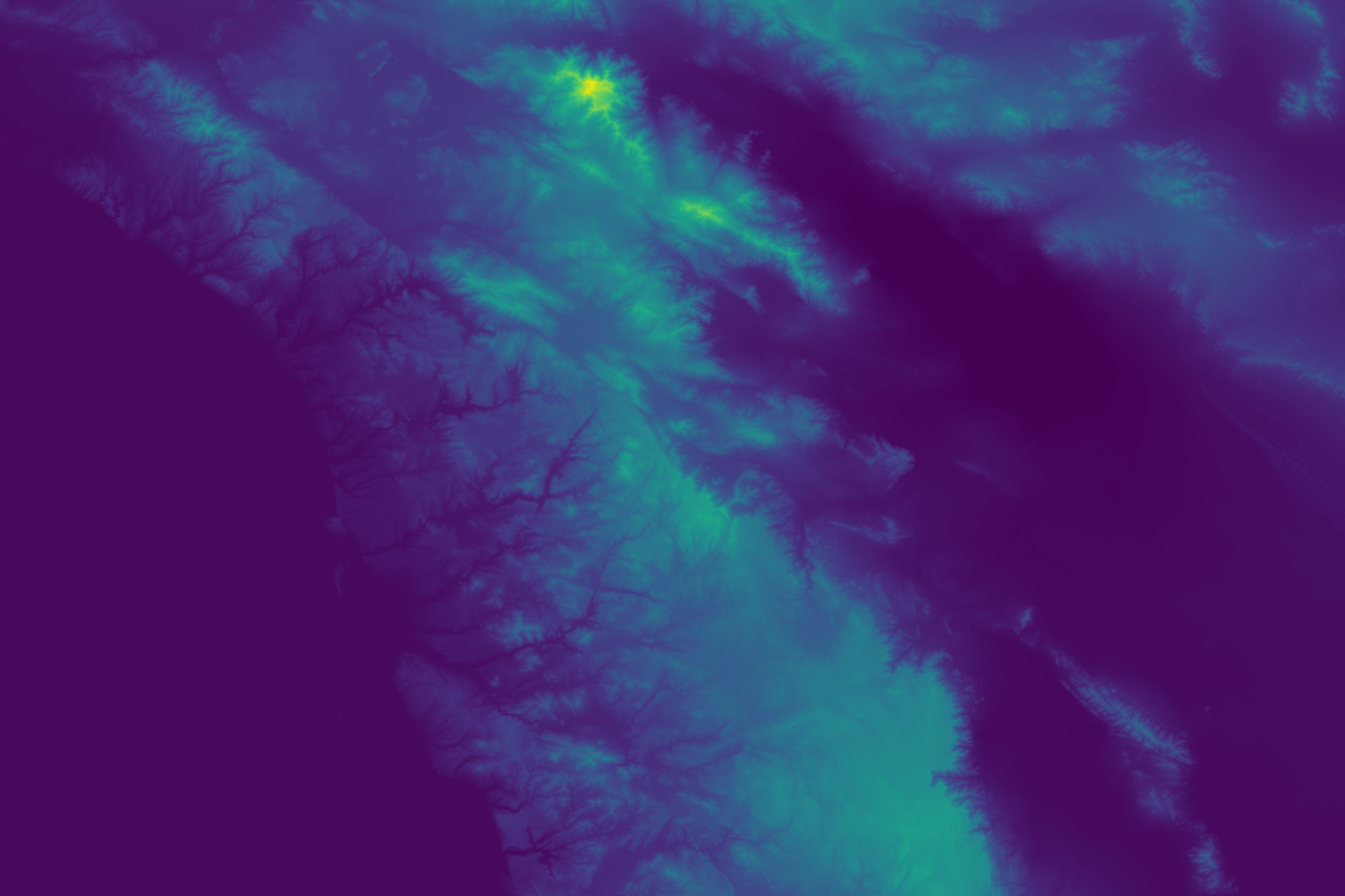
1. Original DEM

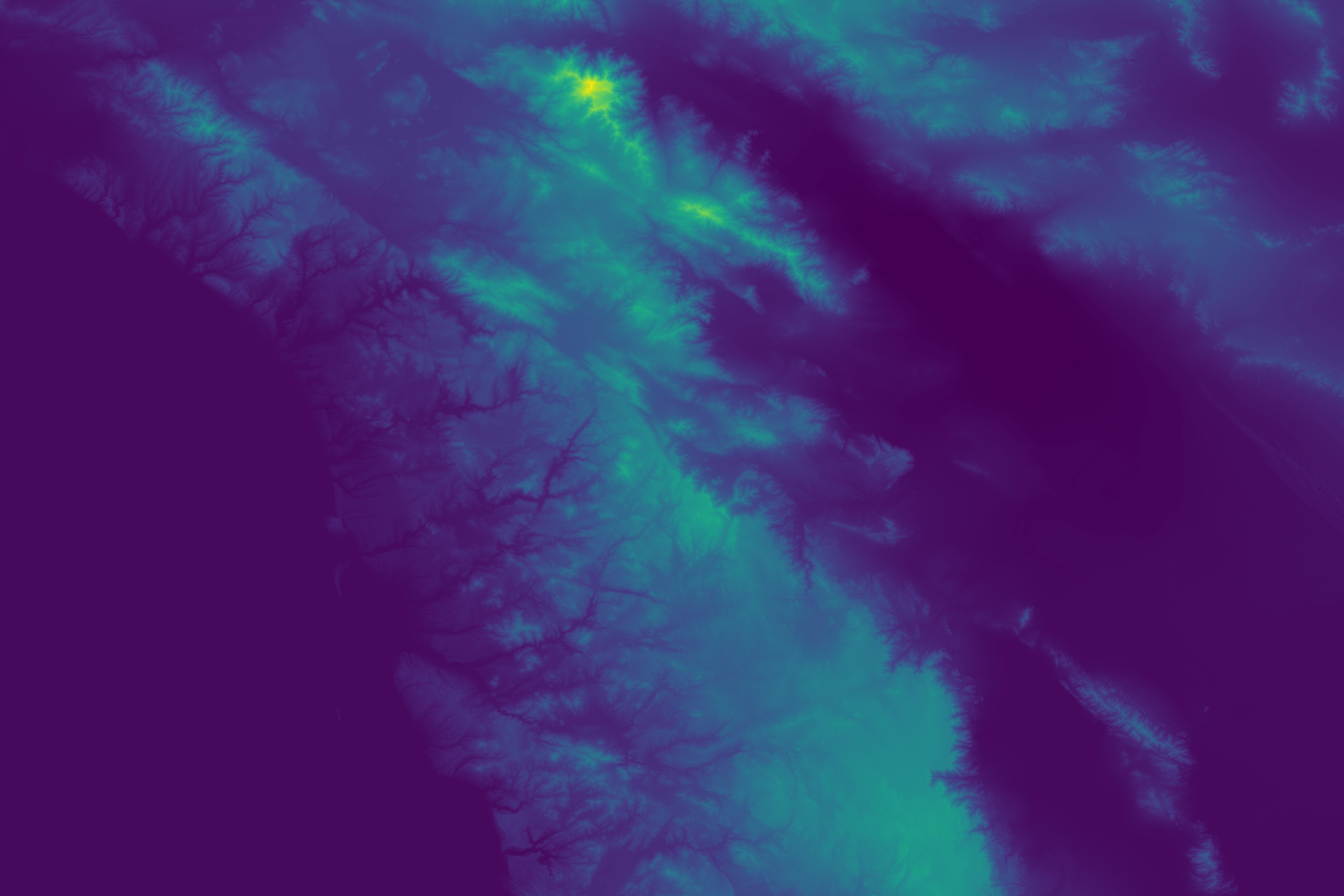
The raw Digital Elevation Model showing terrain elevation. Blue represents ocean/low areas, green/brown shows land elevation gradients.

2. Ocean Mask

Binary mask identifying ocean cells (yellow) vs land cells (purple). Ocean cells act as outlets for coastal drainage.

3. Water Bodies with Inlets/Outlets

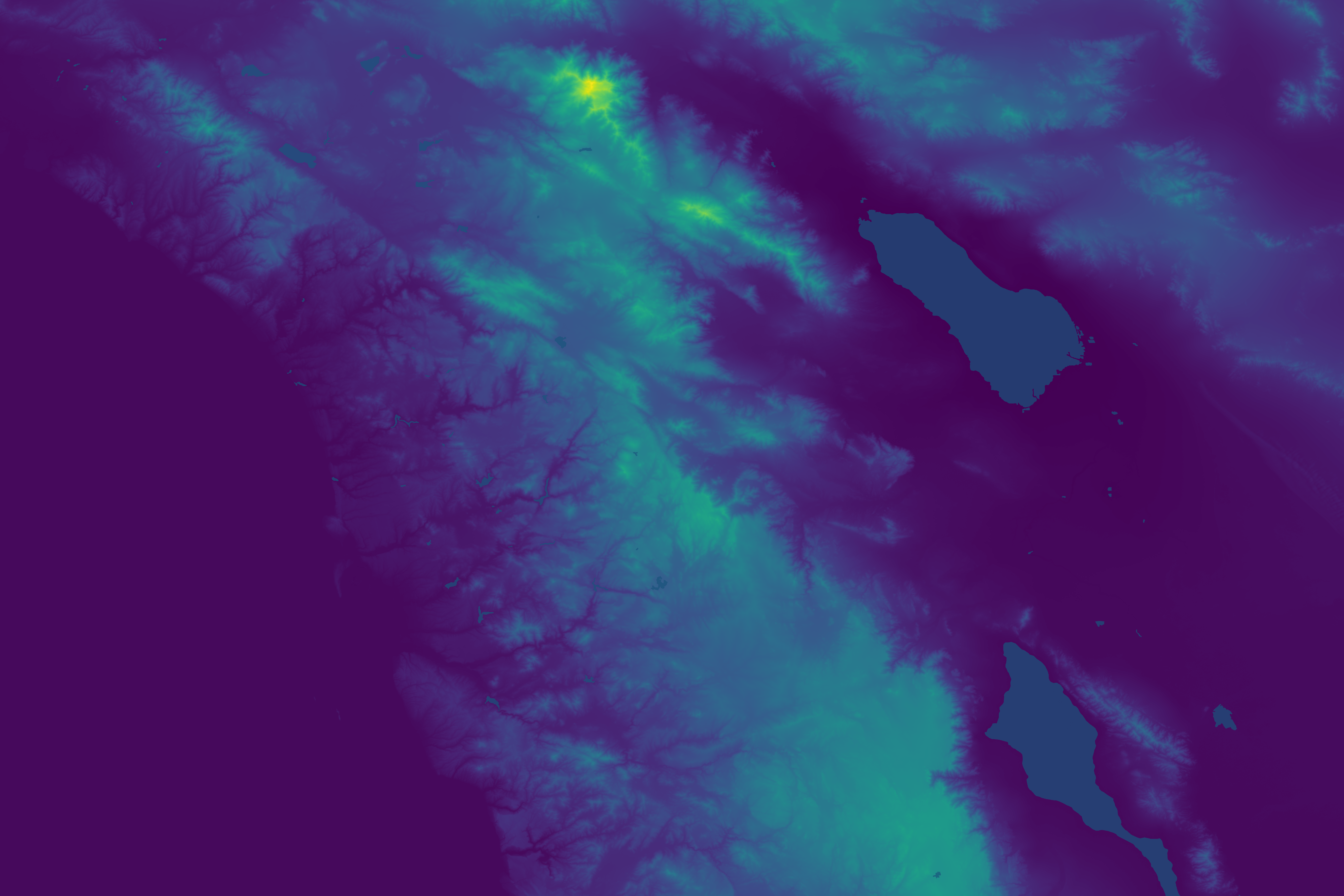
Lakes and reservoirs from HydroLAKES database overlaid on the DEM. Red arrows indicate lake outlets (where water exits), green arrows show inlets (where streams enter lakes).

3b. Endorheic Basins

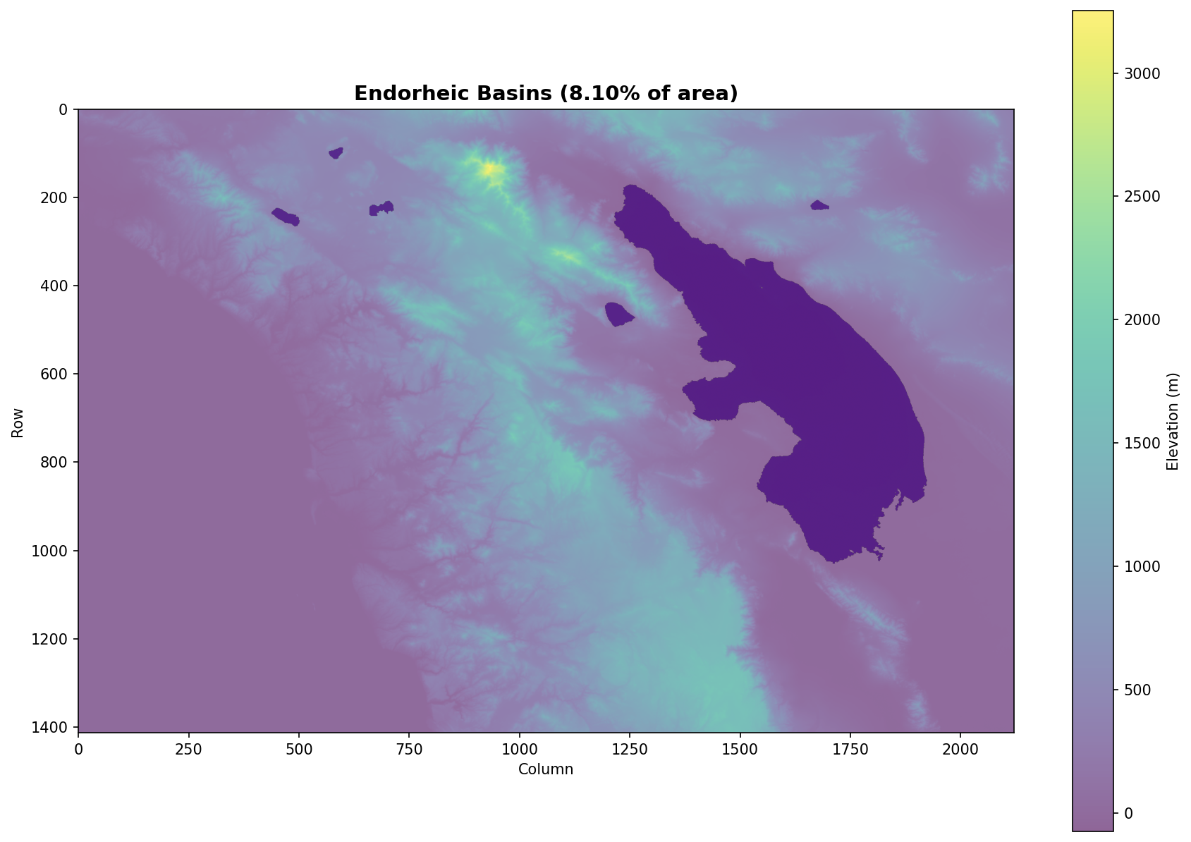
Automatically detected closed drainage basins that don’t drain to the ocean. These are preserved during conditioning to maintain realistic topography.

4. Conditioned DEM

DEM after depression filling/breaching. Artificial sinks have been removed while preserving natural basins and water bodies.

5. Fill Depth

Amount of elevation modification during conditioning (log scale). Lighter colors indicate areas where depressions were filled.

6. D8 Flow Direction

D8 flow direction codes (1-128) showing which neighbor each cell drains to. Different colors represent the 8 possible flow directions.

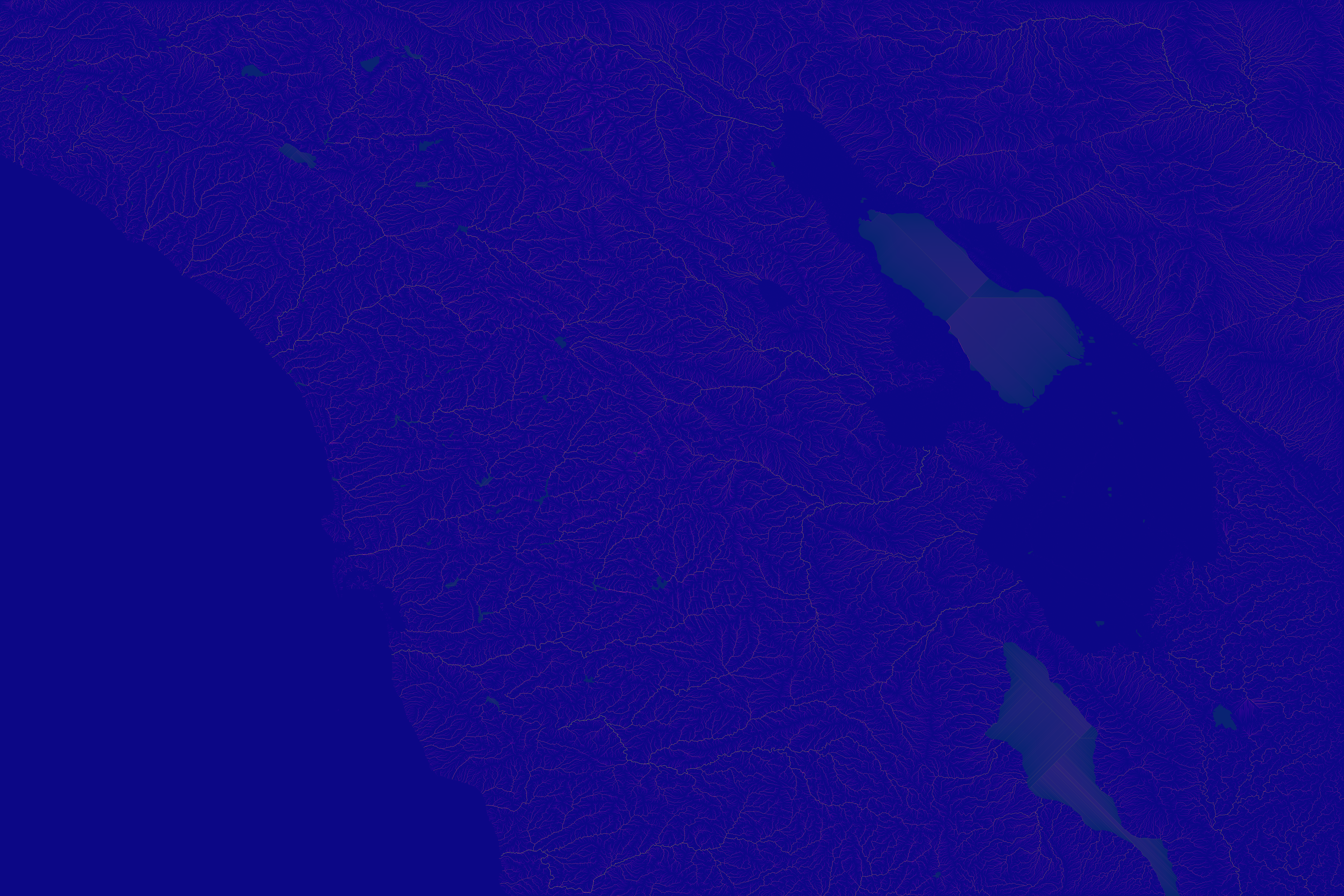
7. Drainage Area

Upstream contributing area for each cell (log scale). Brighter areas have more upstream cells draining through them, revealing the stream network.

8. Stream Network with Lakes

Extracted stream network (top 5% drainage area) overlaid on elevation with lakes highlighted. Shows how streams connect through water bodies.

9. Precipitation

Input precipitation data (synthetic elevation-based or real WorldClim data when available). Used for rainfall-weighted accumulation.

10. Upstream Rainfall

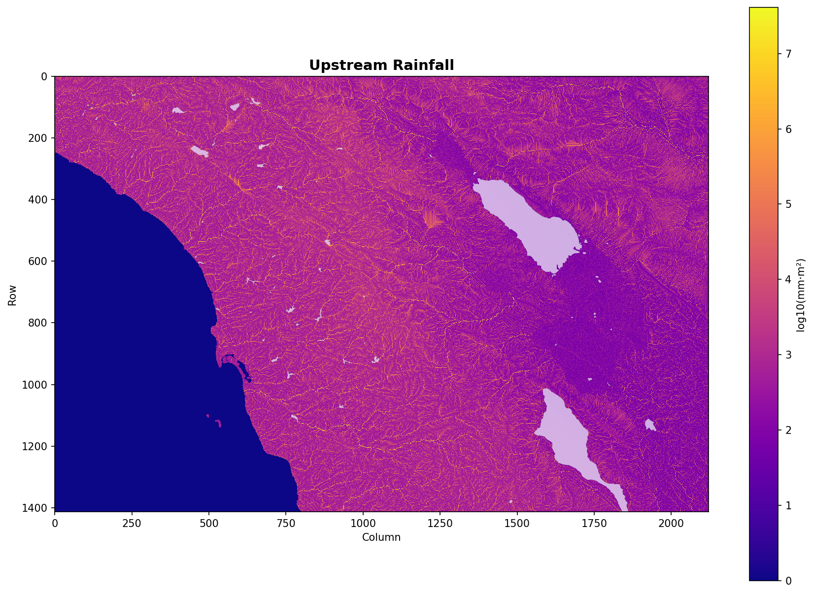
Precipitation-weighted flow accumulation (log scale). Shows total upstream rainfall contributing to each cell.

10b. Discharge Potential (Log Scale)

Combined drainage area and rainfall metric showing potential water discharge. Highlights where the largest flows occur.

10c. Discharge Potential (Linear Scale)

Same discharge metric on linear scale, emphasizing absolute magnitude of major waterways.

11. Validation Summary

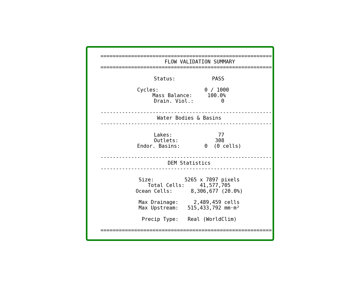
Summary of validation metrics: cycles (should be 0), mass balance (should be >95%), drainage violations, and statistics about water bodies and basins.

Key Observations

1. Water bodies act as conduits: Lakes outside endorheic basins route water through to their outlets, maintaining river connectivity.

2. Endorheic basins preserved: Closed drainage systems are automatically detected and protected from artificial filling.

3. Stream network follows valleys: The extracted network (panel 8) shows realistic dendritic patterns following terrain low points.

4. Mass balance validation: The summary panel confirms no water is lost in the routing process.

---

References

Primary Algorithm Papers

• Barnes, R., Lehman, C., & Mulla, D. (2014). Priority-flood: An optimal depression-filling and watershed-labeling algorithm for digital elevation models. Computers & Geosciences, 62, 117-127.

• Garbrecht, J., & Martz, L.W. (1997). The assignment of drainage direction over flat surfaces in raster digital elevation models. Journal of Hydrology, 193, 204-213.

• Lindsay, J.B. (2016). Efficient hybrid breaching-filling sink removal methods for flow path enforcement in digital elevation models. Hydrological Processes, 30, 846-857.

Classic References

• O’Callaghan, J.F., & Mark, D.M. (1984). The extraction of drainage networks from digital elevation data. Computer Vision, Graphics, and Image Processing, 28, 323-344.

• Jenson, S.K., & Domingue, J.O. (1988). Extracting topographic structure from digital elevation data for geographic information system analysis. Photogrammetric Engineering and Remote Sensing, 54, 1593-1600.

• Tarboton, D.G. (1997). A new method for the determination of flow directions and upslope areas in grid digital elevation models. Water Resources Research, 33, 309-319.

Additional Resources

• Lindsay, J.B., & Creed, I.F. (2005). Removal of artifact depressions from digital elevation models. Hydrological Processes, 19, 3113-3126.

• Barnes, R. (2016). Parallel priority-flood depression filling for trillion cell digital elevation models on desktops or clusters. Computers & Geosciences, 96, 56-68.

---

See Also

• API: flow_accumulation - Function reference