Fit model to participant data
John Flournoy
2020-04-01
fit-model-to-participant-data.RmdMethod
Using the model presented in the section on testing simulated data, I estimate the posterior distribution of the model parameters given the data provided by four groups of participants. Quality of estimation can be supported by (A), (B), (C), (D).
Results
Descriptive plots
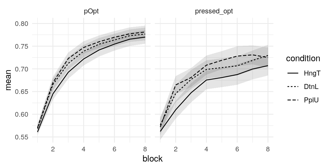
Examination of the raw data using scatterplots and non-parametric best-fit lines can help insure that data conform to expectations, and that subsequent model estimates accurately reflect the data. On average, participants in all samples and all conditions demonstrated learning (Figure @ref(fig:trialaverages)A, although note that given the small sample size, the foster-care involved sample shows more variability across trials). There is also some indication that learning occurs more quickly in the two social motive conditions (Figure @ref(fig:trialaverages)B).
(ref:trialaverages) Average number of optimal responses for each trial across all participants. Best fit lines are generalized additive models with 95% confidence intervals.


Participants also reported their confidence about which reponses would give them rewards most often (this single item measured confidence globally). Confidence generally increases aross trials for all samples (Figure @ref(fig:confidenceplot)).
(ref:confidenceplot) Self-reported confidence over blocks.
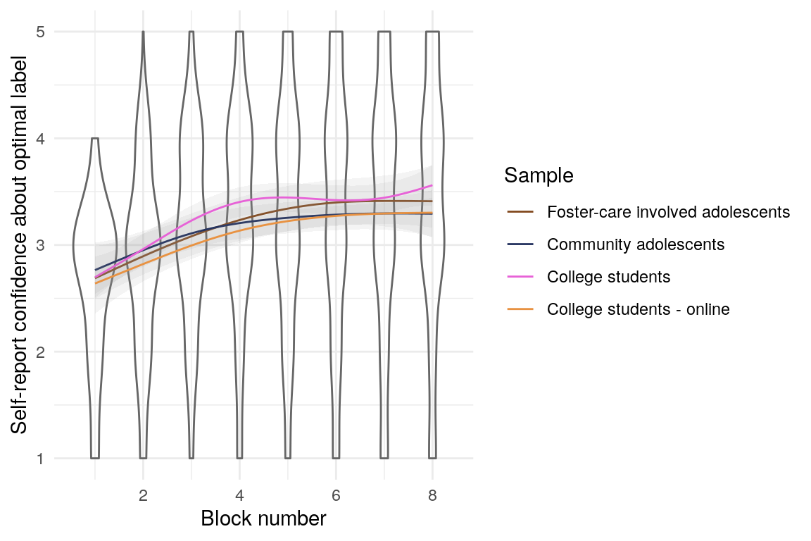
(ref:confidenceplot)
Low-Fi
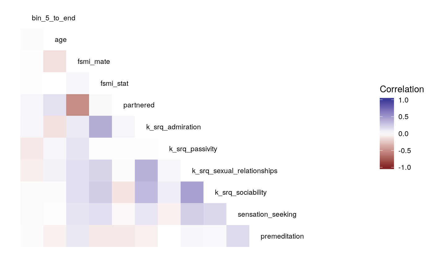
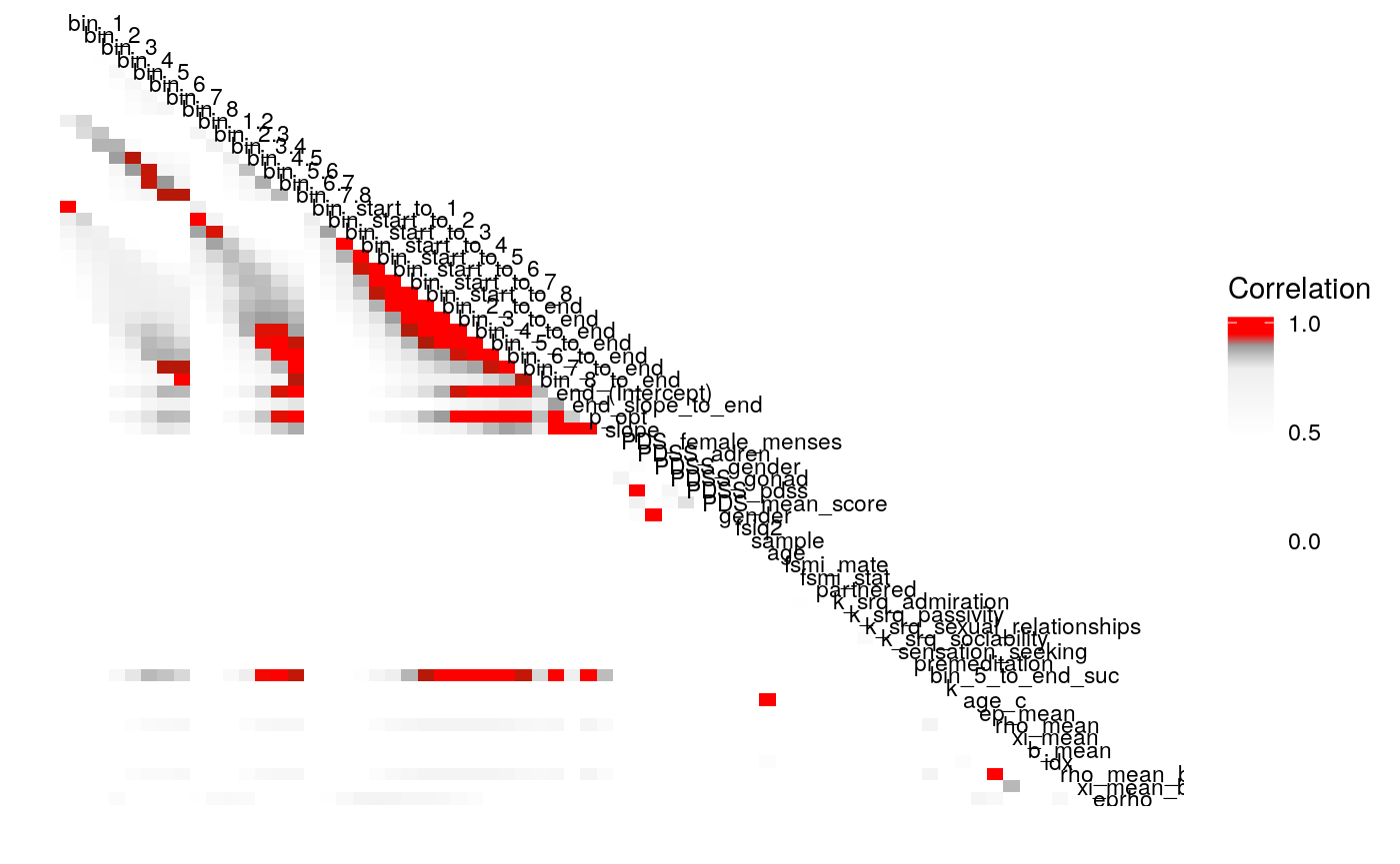
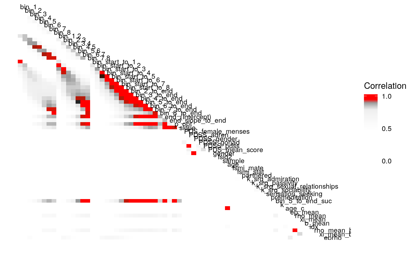
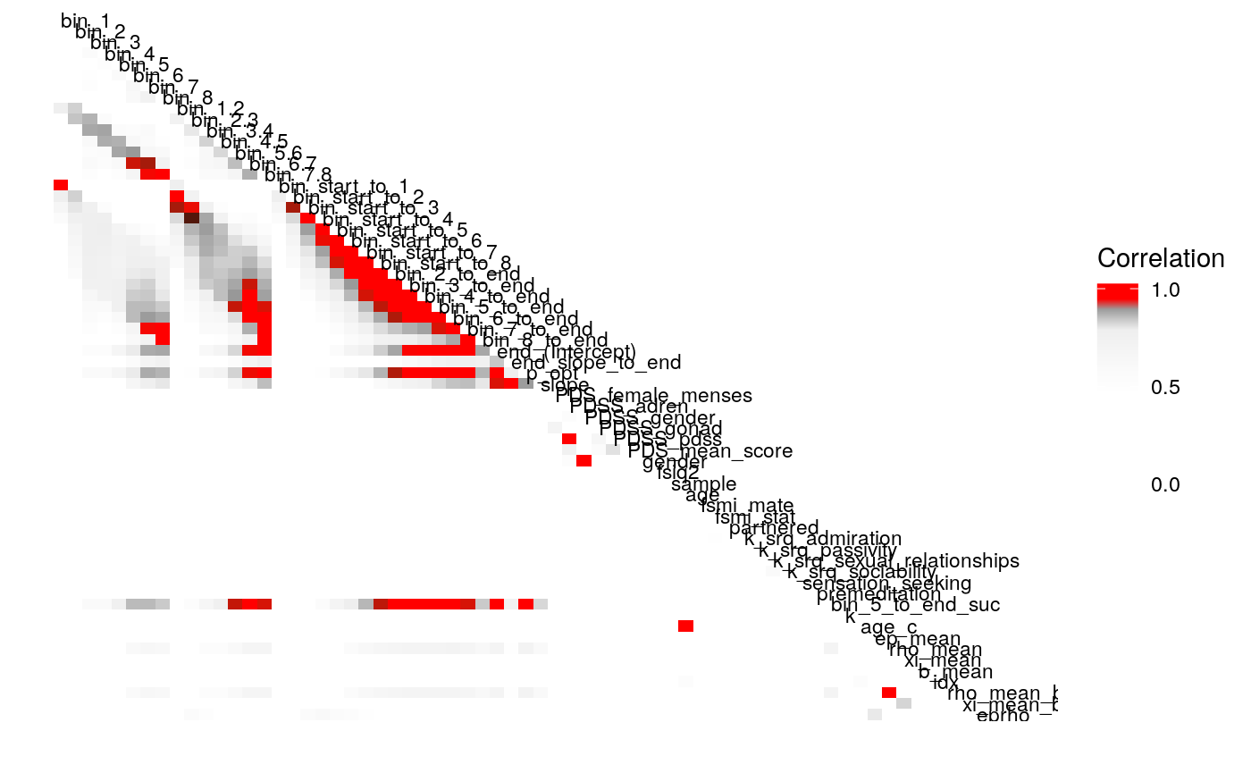
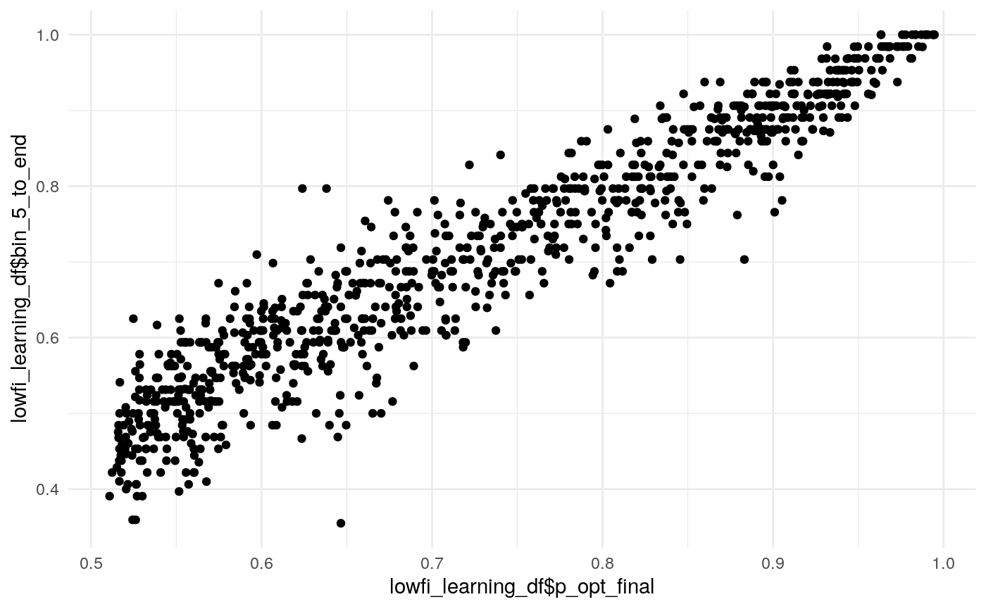
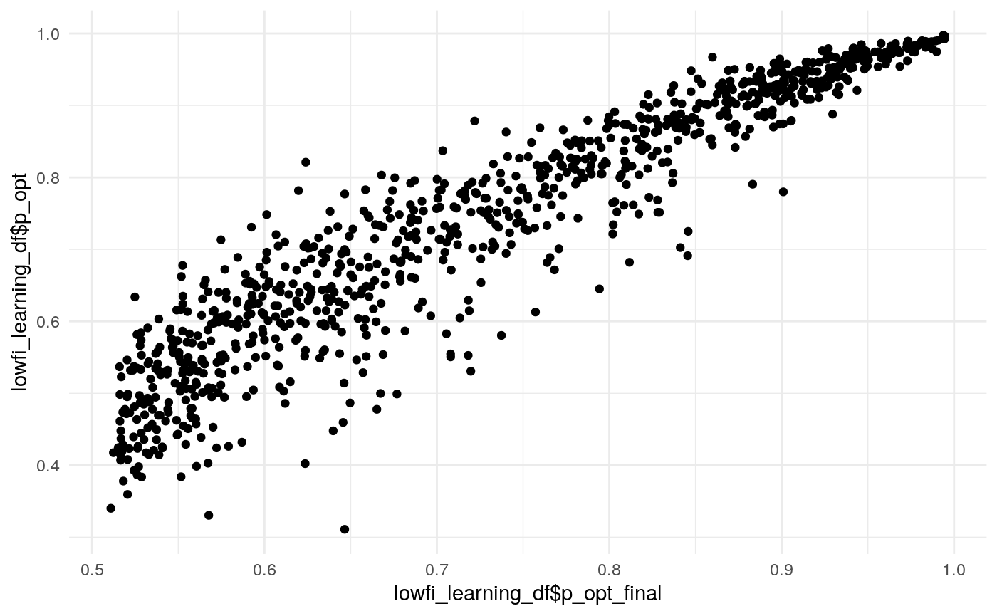
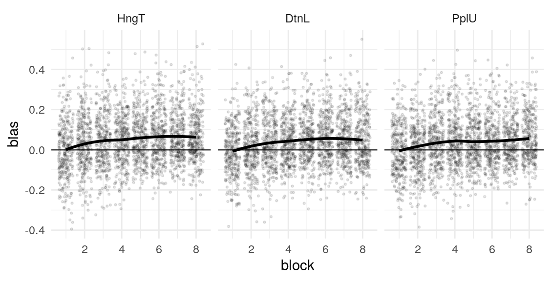
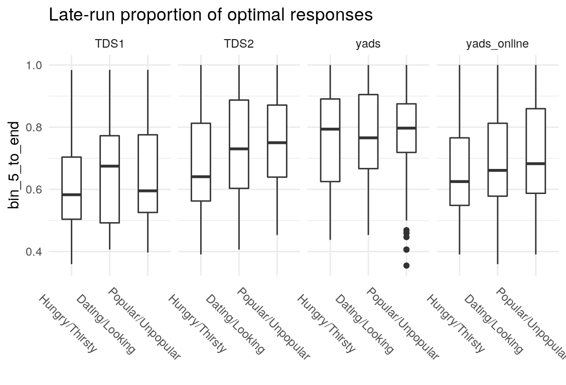
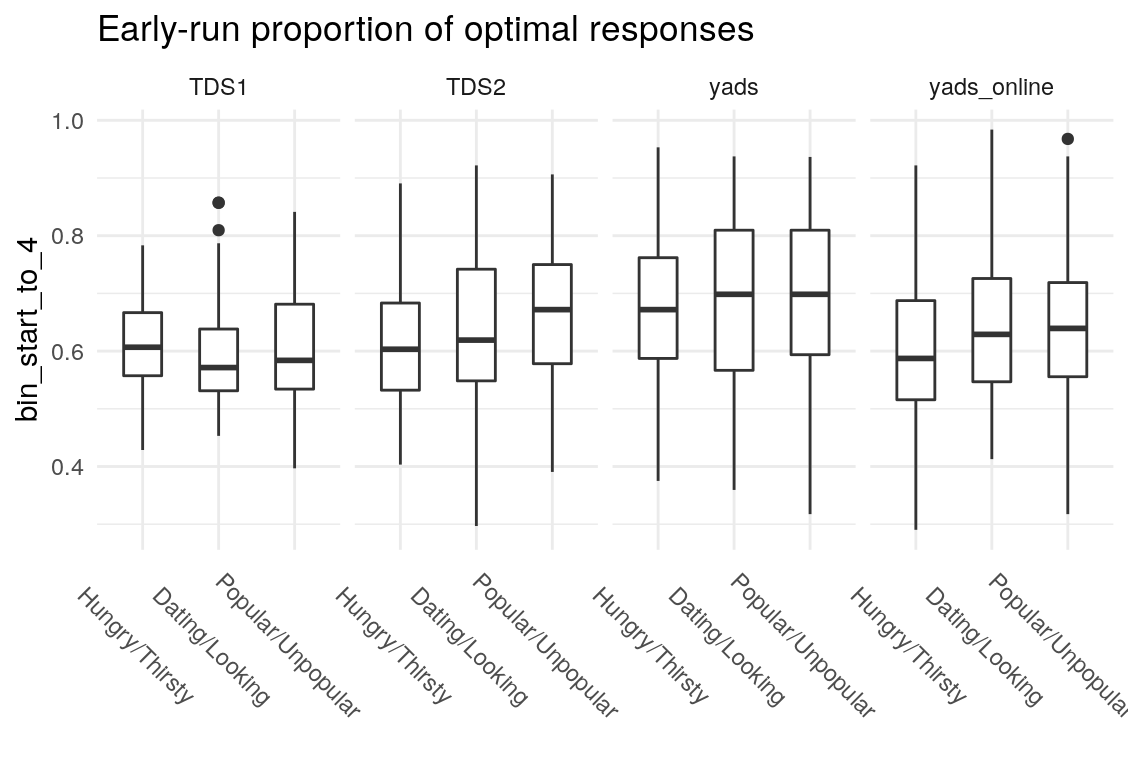
What’s the least sophisticated way I could possibly examine these data? Probably by taking the mean of some subset of the trials in each condition. So let’s do that and see how much stability there is across bins. since there are 128 trials per condition, I split this into bins of 16 trials each, for 8 bins total. I will also create overlapping double bins (e.g., bins 1 and 2, bins 2 and 3) increaslingly large bins starting from the beginning (e.g., combine bins 1 and 2, then bins 1-3), as well as starting from the end (bins 7 and 8, then bins 6-8). In this way, I hope to build up a picture for how much a summary of one subset of bins captures about the rest of the bins. I suspect that bins toward the end of the run will capture more information about the rest of the run than bins at the beginning of the run, as would be consistent with learning throughout the task.
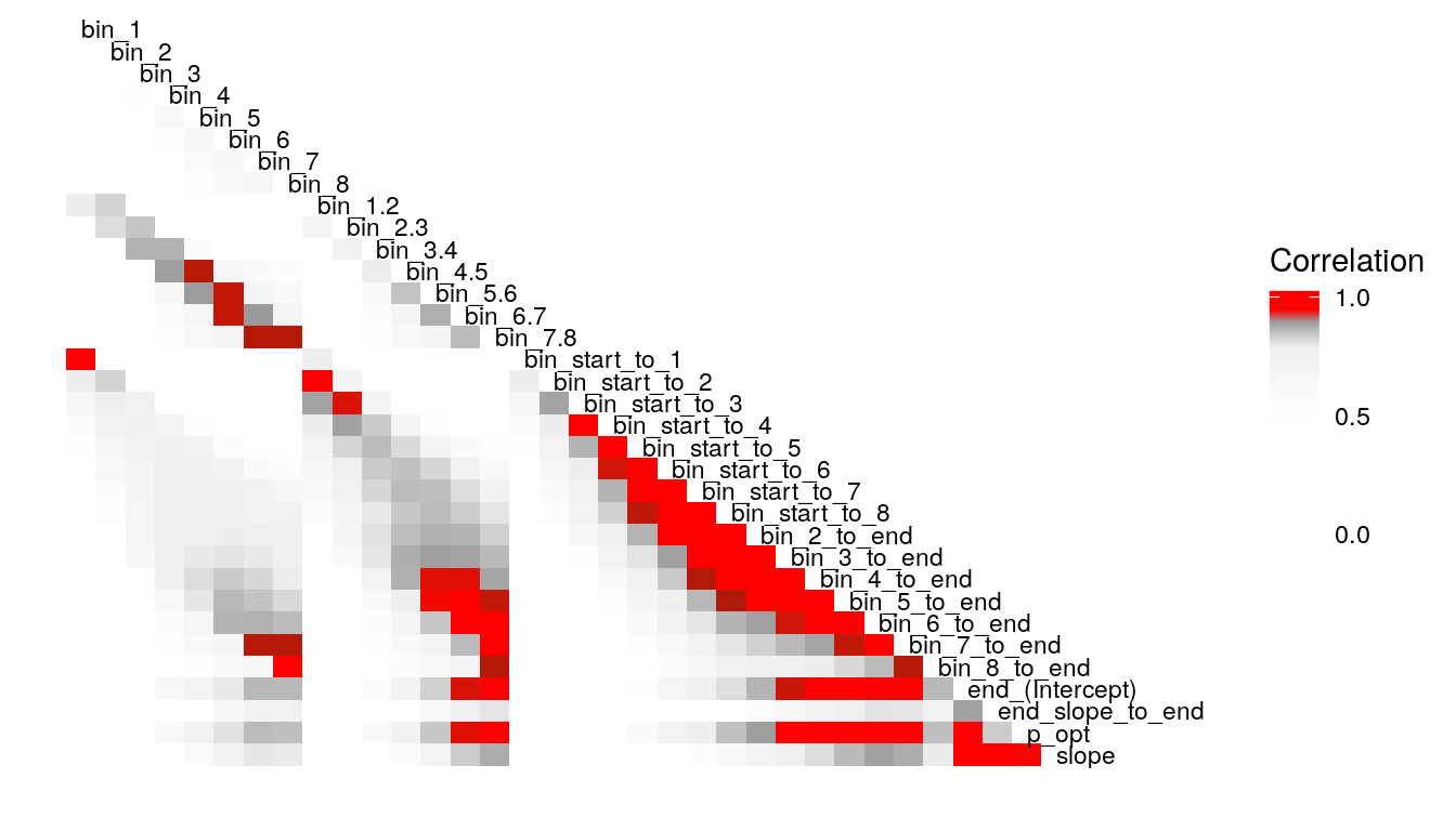
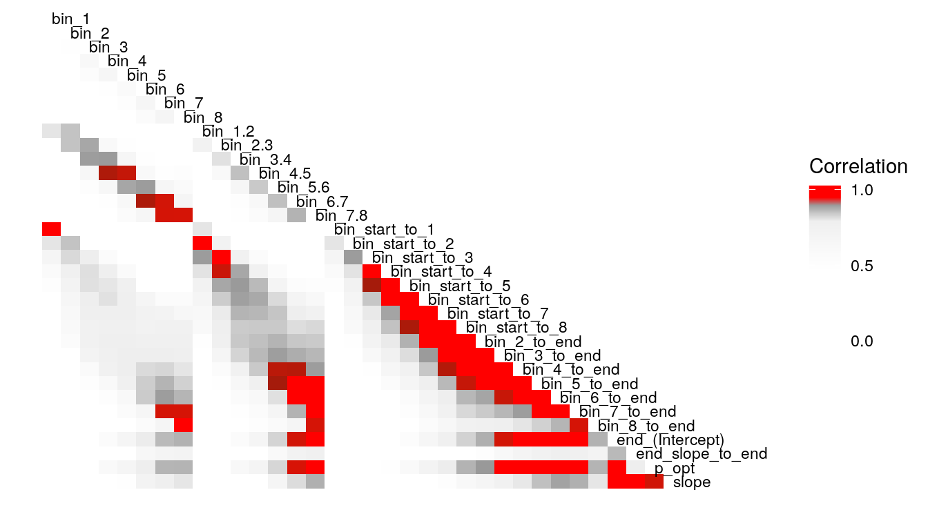

Examining the above plots where corelations r > .90 are colored red (and r = .9 color black), it appears that the most wide ranging correlations are from bins that combine information during the latter half of the run in various ways. If one had to choose such a summary in these data, the average number of optimal presses from bin 5 through 8 (from trial 65 through trial 128) seems like a good candidate. It is highly correlated with average optimal responding from bin 6-end and 7-end, combined bins 5 & 6, combined bins 6 & 7, as well as the combined bins from start to finish (“bin_start_to_8”). Using the intercept from a logistic regression with the trial number predictor centered toward the end of the trial also captures a good deal of variance that corresponds to optimal responding on trials toward the end of the run.
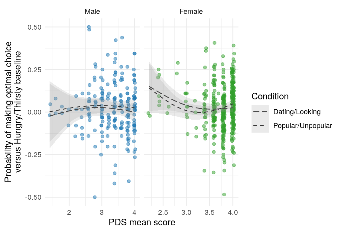
Age and dev
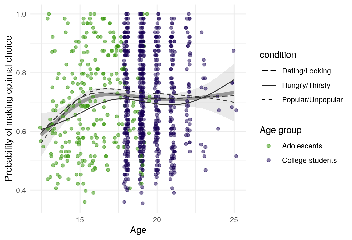
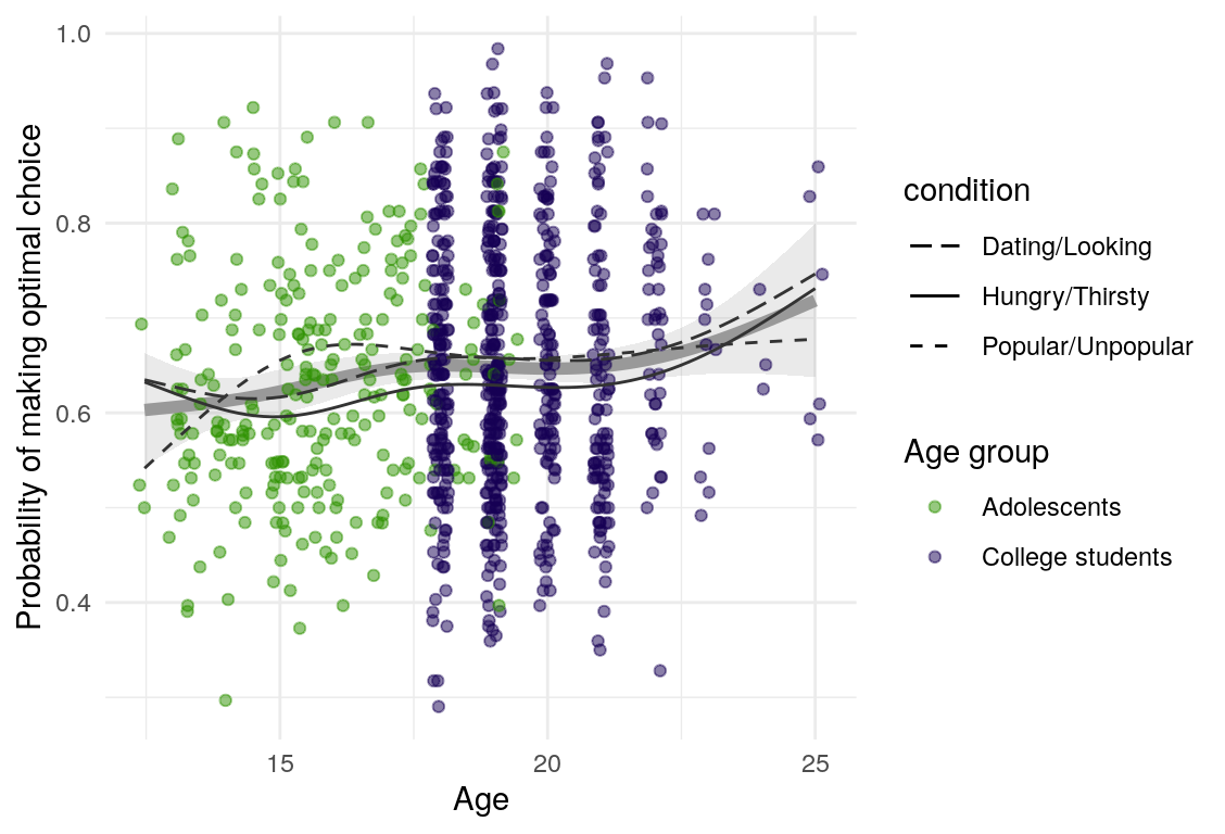
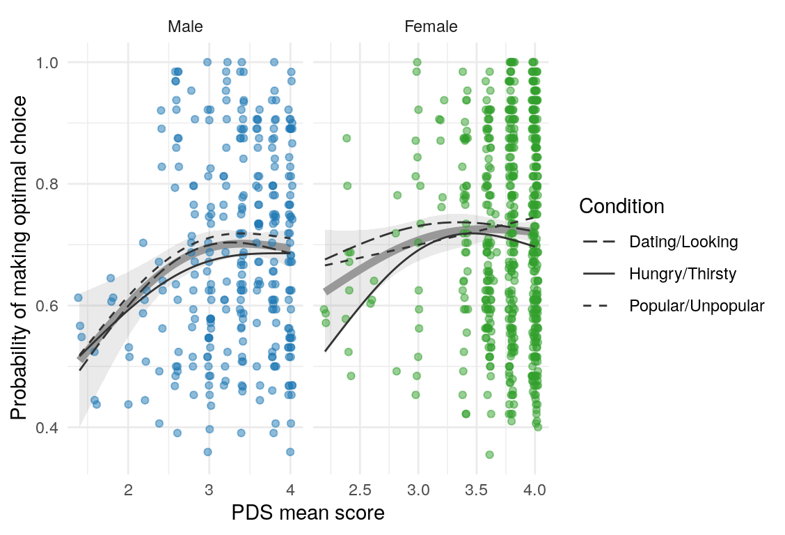
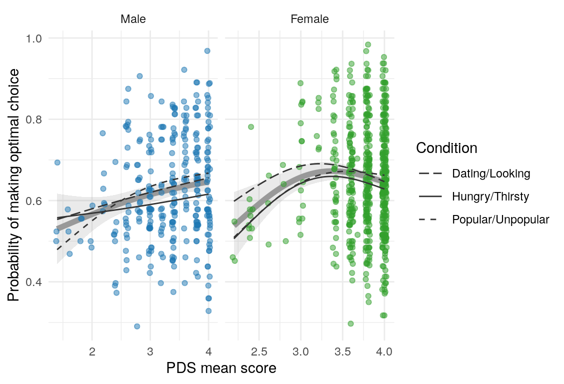
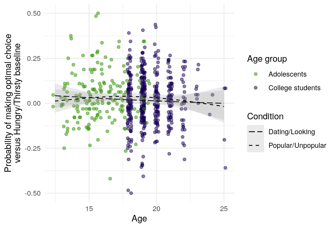
Here are a few plots of these parameters against age.
| Variables | Age-group | \(\beta\) | \(\text{SE}_{\beta}\) | \(t\) |
|---|---|---|---|---|
| Optimal choices \(\sim\) Age | Adolescent | 0.17 | 0.09 | 1.87 |
| Optimal choices \(\sim\) Age | College | 0.00 | 0.06 | 0.02 |
| Optimal choices \(\sim\) Age | All | 0.07 | 0.05 | 1.48 |
| Optimal choices \(\sim\) PDS | Adolescent | 0.17 | 0.09 | 1.85 |
| Optimal choices \(\sim\) PDS | College | 0.09 | 0.06 | 1.45 |
| Optimal choices \(\sim\) PDS | All | 0.12 | 0.05 | 2.49 |
| Optimal choices contrasts \(\sim\) Age | Adolescent | 0.08 | 0.10 | 0.82 |
| Optimal choices contrasts \(\sim\) Age | College | 0.01 | 0.06 | 0.15 |
| Optimal choices contrasts \(\sim\) Age | All | -0.03 | 0.05 | -0.67 |
| Optimal choices contrasts \(\sim\) PDS | Adolescent | 0.03 | 0.10 | 0.29 |
| Optimal choices contrasts \(\sim\) PDS | College | 0.02 | 0.06 | 0.27 |
| Optimal choices contrasts \(\sim\) PDS | All | -0.01 | 0.05 | -0.22 |
| Variables | Age-group | \(\beta\) | \(\text{SE}_{\beta}\) | \(t\) |
|---|---|---|---|---|
| Optimal choices \(\sim\) Age | Adolescent | 0.11 | 0.08 | 1.37 |
| Optimal choices \(\sim\) Age | College | 0.03 | 0.05 | 0.66 |
| Optimal choices \(\sim\) Age | All | 0.09 | 0.04 | 2.11 |
| Optimal choices \(\sim\) PDS | Adolescent | 0.16 | 0.08 | 1.95 |
| Optimal choices \(\sim\) PDS | College | 0.09 | 0.05 | 1.81 |
| Optimal choices \(\sim\) PDS | All | 0.13 | 0.04 | 2.99 |
| Optimal choices contrasts \(\sim\) Age | Adolescent | -0.01 | 0.09 | -0.07 |
| Optimal choices contrasts \(\sim\) Age | College | -0.03 | 0.06 | -0.54 |
| Optimal choices contrasts \(\sim\) Age | All | 0.00 | 0.05 | 0.07 |
| Optimal choices contrasts \(\sim\) PDS | Adolescent | 0.03 | 0.09 | 0.31 |
| Optimal choices contrasts \(\sim\) PDS | College | 0.00 | 0.06 | -0.06 |
| Optimal choices contrasts \(\sim\) PDS | All | 0.02 | 0.05 | 0.38 |
Dating/Looking
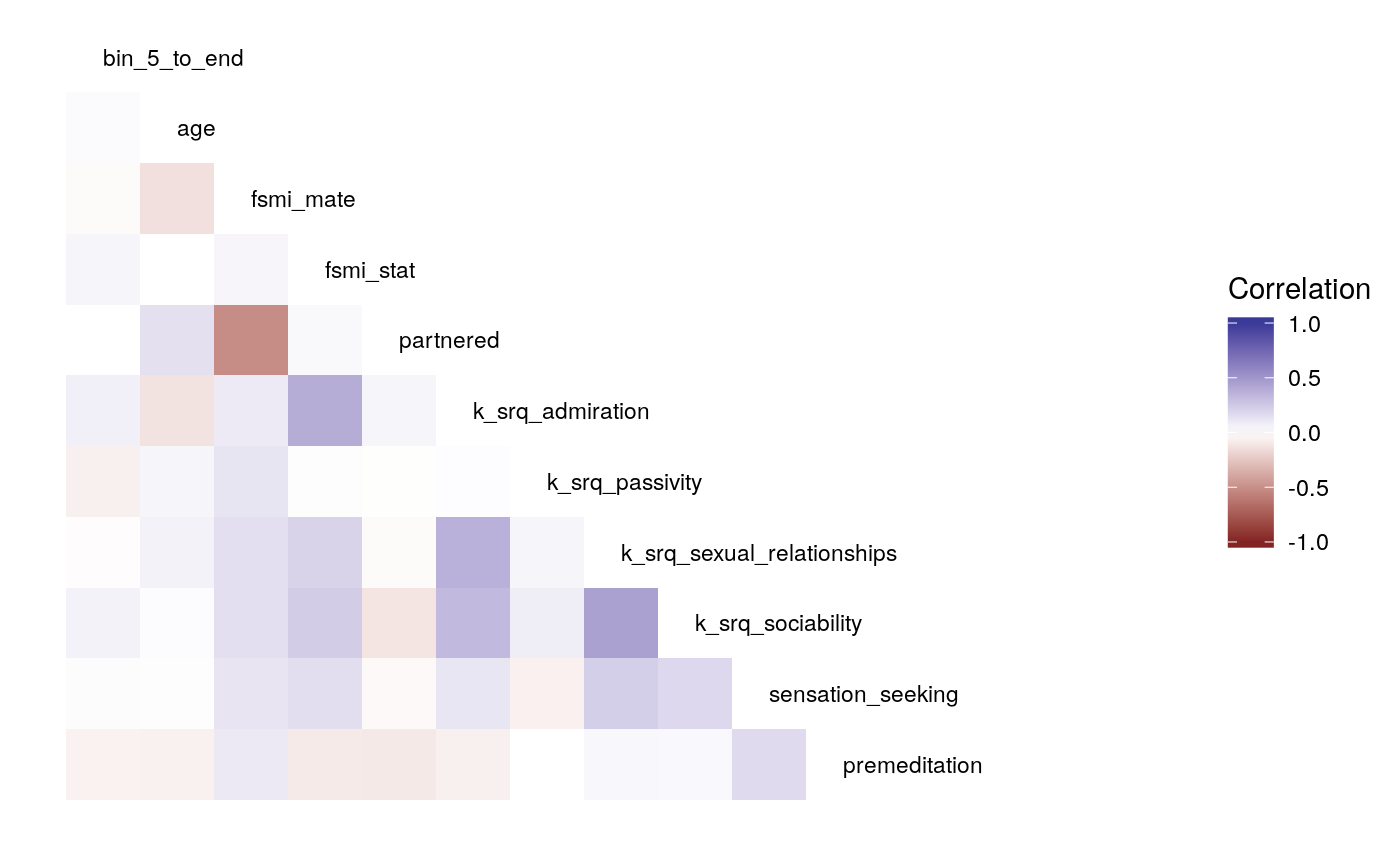
Diff
#>
#>
#> bin_5_to_end age fsmi_mate fsmi_stat partnered k_srq_admiration k_srq_passivity k_srq_sexual_relationships k_srq_sociability sensation_seeking premeditation
#> --------------------------- ------------- ------- ---------- ---------- ---------- ----------------- ---------------- --------------------------- ------------------ ------------------ --------------
#> bin_5_to_end 1.000 -0.018 0.005 0.007 0.042 0.046 -0.103 -0.072 -0.019 0.021 -0.016
#> age -0.018 1.000 -0.137 -0.002 0.145 -0.127 0.046 0.058 0.018 0.008 -0.061
#> fsmi_mate 0.005 -0.137 1.000 0.045 -0.515 0.095 0.121 0.151 0.147 0.124 0.102
#> fsmi_stat 0.007 -0.002 0.045 1.000 0.029 0.388 -0.010 0.203 0.238 0.155 -0.093
#> partnered 0.042 0.145 -0.515 0.029 1.000 0.047 -0.006 -0.021 -0.113 -0.028 -0.098
#> k_srq_admiration 0.046 -0.127 0.095 0.388 0.047 1.000 0.012 0.370 0.326 0.117 -0.066
#> k_srq_passivity -0.103 0.046 0.121 -0.010 -0.006 0.012 1.000 0.048 0.084 -0.065 -0.001
#> k_srq_sexual_relationships -0.072 0.058 0.151 0.203 -0.021 0.370 0.048 1.000 0.446 0.227 0.037
#> k_srq_sociability -0.019 0.018 0.147 0.238 -0.113 0.326 0.084 0.446 1.000 0.180 0.030
#> sensation_seeking 0.021 0.008 0.124 0.155 -0.028 0.117 -0.065 0.227 0.180 1.000 0.172
#> premeditation -0.016 -0.061 0.102 -0.093 -0.098 -0.066 -0.001 0.037 0.030 0.172 1.000
#>
#>
#> bin_5_to_end age fsmi_mate fsmi_stat partnered k_srq_admiration k_srq_passivity k_srq_sexual_relationships k_srq_sociability sensation_seeking premeditation
#> --------------------------- ------------- ------ ---------- ---------- ---------- ----------------- ---------------- --------------------------- ------------------ ------------------ --------------
#> bin_5_to_end 0.000 1.000 1.000 1.000 1.000 1.000 1.000 1.000 1.000 1.000 1.000
#> age 0.751 0.000 1.000 1.000 1.000 1.000 1.000 1.000 1.000 1.000 1.000
#> fsmi_mate 0.944 0.042 0.000 1.000 0.000 1.000 1.000 1.000 1.000 1.000 1.000
#> fsmi_stat 0.920 0.982 0.511 0.000 1.000 0.000 1.000 0.125 0.020 1.000 1.000
#> partnered 0.535 0.032 0.000 0.666 0.000 1.000 1.000 1.000 1.000 1.000 1.000
#> k_srq_admiration 0.423 0.027 0.161 0.000 0.495 0.000 1.000 0.000 0.000 1.000 1.000
#> k_srq_passivity 0.074 0.423 0.076 0.887 0.927 0.834 0.000 1.000 1.000 1.000 1.000
#> k_srq_sexual_relationships 0.212 0.312 0.026 0.003 0.754 0.000 0.407 0.000 0.000 0.007 1.000
#> k_srq_sociability 0.738 0.751 0.031 0.000 0.097 0.000 0.143 0.000 0.000 0.127 1.000
#> sensation_seeking 0.727 0.892 0.086 0.031 0.701 0.052 0.285 0.000 0.003 0.000 0.181
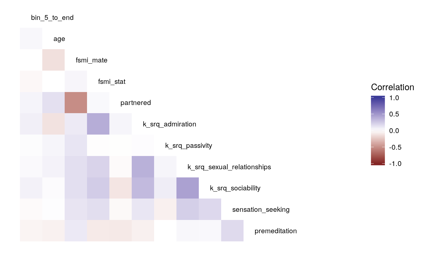
#> premeditation 0.794 0.312 0.157 0.200 0.177 0.276 0.991 0.538 0.615 0.004 0.000Raw
#>
#>
#> bin_5_to_end age fsmi_mate fsmi_stat partnered k_srq_admiration k_srq_passivity k_srq_sexual_relationships k_srq_sociability sensation_seeking premeditation
#> --------------------------- ------------- ------- ---------- ---------- ---------- ----------------- ---------------- --------------------------- ------------------ ------------------ --------------
#> bin_5_to_end 1.000 0.019 -0.022 0.048 -0.001 0.073 -0.066 -0.012 0.061 0.016 -0.058
#> age 0.019 1.000 -0.137 -0.002 0.145 -0.127 0.046 0.058 0.018 0.008 -0.061
#> fsmi_mate -0.022 -0.137 1.000 0.045 -0.515 0.095 0.121 0.151 0.147 0.124 0.102
#> fsmi_stat 0.048 -0.002 0.045 1.000 0.029 0.388 -0.010 0.203 0.238 0.155 -0.093
#> partnered -0.001 0.145 -0.515 0.029 1.000 0.047 -0.006 -0.021 -0.113 -0.028 -0.098
#> k_srq_admiration 0.073 -0.127 0.095 0.388 0.047 1.000 0.012 0.370 0.326 0.117 -0.066
#> k_srq_passivity -0.066 0.046 0.121 -0.010 -0.006 0.012 1.000 0.048 0.084 -0.065 -0.001
#> k_srq_sexual_relationships -0.012 0.058 0.151 0.203 -0.021 0.370 0.048 1.000 0.446 0.227 0.037
#> k_srq_sociability 0.061 0.018 0.147 0.238 -0.113 0.326 0.084 0.446 1.000 0.180 0.030
#> sensation_seeking 0.016 0.008 0.124 0.155 -0.028 0.117 -0.065 0.227 0.180 1.000 0.172
#> premeditation -0.058 -0.061 0.102 -0.093 -0.098 -0.066 -0.001 0.037 0.030 0.172 1.000
#>
#>
#> bin_5_to_end age fsmi_mate fsmi_stat partnered k_srq_admiration k_srq_passivity k_srq_sexual_relationships k_srq_sociability sensation_seeking premeditation
#> --------------------------- ------------- ------ ---------- ---------- ---------- ----------------- ---------------- --------------------------- ------------------ ------------------ --------------
#> bin_5_to_end 0.000 1.000 1.000 1.000 1.000 1.000 1.000 1.000 1.000 1.000 1.000
#> age 0.734 0.000 1.000 1.000 1.000 1.000 1.000 1.000 1.000 1.000 1.000
#> fsmi_mate 0.750 0.042 0.000 1.000 0.000 1.000 1.000 1.000 1.000 1.000 1.000
#> fsmi_stat 0.482 0.982 0.511 0.000 1.000 0.000 1.000 0.125 0.020 1.000 1.000
#> partnered 0.983 0.032 0.000 0.666 0.000 1.000 1.000 1.000 1.000 1.000 1.000
#> k_srq_admiration 0.207 0.027 0.161 0.000 0.495 0.000 1.000 0.000 0.000 1.000 1.000
#> k_srq_passivity 0.250 0.423 0.076 0.887 0.927 0.834 0.000 1.000 1.000 1.000 1.000
#> k_srq_sexual_relationships 0.831 0.312 0.026 0.003 0.754 0.000 0.407 0.000 0.000 0.007 1.000
#> k_srq_sociability 0.286 0.751 0.031 0.000 0.097 0.000 0.143 0.000 0.000 0.127 1.000
#> sensation_seeking 0.791 0.892 0.086 0.031 0.701 0.052 0.285 0.000 0.003 0.000 0.181
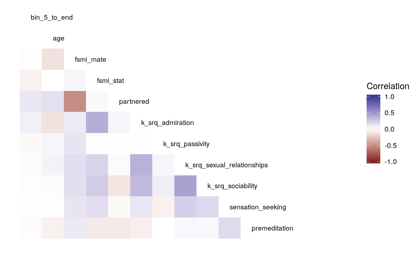
#> premeditation 0.337 0.312 0.157 0.200 0.177 0.276 0.991 0.538 0.615 0.004 0.000Popular/Unpopular
#>
#>
#>                               bin_5_to_end      age   fsmi_mate   fsmi_stat   partnered   k_srq_admiration   k_srq_passivity   k_srq_sexual_relationships   k_srq_sociability   sensation_seeking   premeditation
#> ---------------------------  -------------  -------  ----------  ----------  ----------  -----------------  ----------------  ---------------------------  ------------------  ------------------  --------------
#> bin_5_to_end                         1.000   -0.018       0.005       0.007       0.042              0.046            -0.103                       -0.072              -0.019               0.021          -0.016
#> age                                 -0.018    1.000      -0.137      -0.002       0.145             -0.127             0.046                        0.058               0.018               0.008          -0.061
#> fsmi_mate                            0.005   -0.137       1.000       0.045      -0.515              0.095             0.121                        0.151               0.147               0.124           0.102
#> fsmi_stat                            0.007   -0.002       0.045       1.000       0.029              0.388            -0.010                        0.203               0.238               0.155          -0.093
#> partnered                            0.042    0.145      -0.515       0.029       1.000              0.047            -0.006                       -0.021              -0.113              -0.028          -0.098
#> k_srq_admiration                     0.046   -0.127       0.095       0.388       0.047              1.000             0.012                        0.370               0.326               0.117          -0.066
#> k_srq_passivity                     -0.103    0.046       0.121      -0.010      -0.006              0.012             1.000                        0.048               0.084              -0.065          -0.001
#> k_srq_sexual_relationships          -0.072    0.058       0.151       0.203      -0.021              0.370             0.048                        1.000               0.446               0.227           0.037
#> k_srq_sociability                   -0.019    0.018       0.147       0.238      -0.113              0.326             0.084                        0.446               1.000               0.180           0.030
#> sensation_seeking                    0.021    0.008       0.124       0.155      -0.028              0.117            -0.065                        0.227               0.180               1.000           0.172
#> premeditation                       -0.016   -0.061       0.102      -0.093      -0.098             -0.066            -0.001                        0.037               0.030               0.172           1.000
#>
#>
#>                               bin_5_to_end     age   fsmi_mate   fsmi_stat   partnered   k_srq_admiration   k_srq_passivity   k_srq_sexual_relationships   k_srq_sociability   sensation_seeking   premeditation
#> ---------------------------  -------------  ------  ----------  ----------  ----------  -----------------  ----------------  ---------------------------  ------------------  ------------------  --------------
#> bin_5_to_end                         0.000   1.000       1.000       1.000       1.000              1.000             1.000                        1.000               1.000               1.000           1.000
#> age                                  0.751   0.000       1.000       1.000       1.000              1.000             1.000                        1.000               1.000               1.000           1.000
#> fsmi_mate                            0.944   0.042       0.000       1.000       0.000              1.000             1.000                        1.000               1.000               1.000           1.000
#> fsmi_stat                            0.920   0.982       0.511       0.000       1.000              0.000             1.000                        0.125               0.020               1.000           1.000
#> partnered                            0.535   0.032       0.000       0.666       0.000              1.000             1.000                        1.000               1.000               1.000           1.000
#> k_srq_admiration                     0.423   0.027       0.161       0.000       0.495              0.000             1.000                        0.000               0.000               1.000           1.000
#> k_srq_passivity                      0.074   0.423       0.076       0.887       0.927              0.834             0.000                        1.000               1.000               1.000           1.000
#> k_srq_sexual_relationships           0.212   0.312       0.026       0.003       0.754              0.000             0.407                        0.000               0.000               0.007           1.000
#> k_srq_sociability                    0.738   0.751       0.031       0.000       0.097              0.000             0.143                        0.000               0.000               0.127           1.000
#> sensation_seeking                    0.727   0.892       0.086       0.031       0.701              0.052             0.285                        0.000               0.003               0.000           0.181
#> premeditation                        0.794   0.312       0.157       0.200       0.177              0.276             0.991                        0.538               0.615               0.004           0.000
Raw
#>
#>
#>                               bin_5_to_end      age   fsmi_mate   fsmi_stat   partnered   k_srq_admiration   k_srq_passivity   k_srq_sexual_relationships   k_srq_sociability   sensation_seeking   premeditation
#> ---------------------------  -------------  -------  ----------  ----------  ----------  -----------------  ----------------  ---------------------------  ------------------  ------------------  --------------
#> bin_5_to_end                         1.000    0.019      -0.022       0.048      -0.001              0.073            -0.066                       -0.012               0.061               0.016          -0.058
#> age                                  0.019    1.000      -0.137      -0.002       0.145             -0.127             0.046                        0.058               0.018               0.008          -0.061
#> fsmi_mate                           -0.022   -0.137       1.000       0.045      -0.515              0.095             0.121                        0.151               0.147               0.124           0.102
#> fsmi_stat                            0.048   -0.002       0.045       1.000       0.029              0.388            -0.010                        0.203               0.238               0.155          -0.093
#> partnered                           -0.001    0.145      -0.515       0.029       1.000              0.047            -0.006                       -0.021              -0.113              -0.028          -0.098
#> k_srq_admiration                     0.073   -0.127       0.095       0.388       0.047              1.000             0.012                        0.370               0.326               0.117          -0.066
#> k_srq_passivity                     -0.066    0.046       0.121      -0.010      -0.006              0.012             1.000                        0.048               0.084              -0.065          -0.001
#> k_srq_sexual_relationships          -0.012    0.058       0.151       0.203      -0.021              0.370             0.048                        1.000               0.446               0.227           0.037
#> k_srq_sociability                    0.061    0.018       0.147       0.238      -0.113              0.326             0.084                        0.446               1.000               0.180           0.030
#> sensation_seeking                    0.016    0.008       0.124       0.155      -0.028              0.117            -0.065                        0.227               0.180               1.000           0.172
#> premeditation                       -0.058   -0.061       0.102      -0.093      -0.098             -0.066            -0.001                        0.037               0.030               0.172           1.000
#>
#>
#>                               bin_5_to_end     age   fsmi_mate   fsmi_stat   partnered   k_srq_admiration   k_srq_passivity   k_srq_sexual_relationships   k_srq_sociability   sensation_seeking   premeditation
#> ---------------------------  -------------  ------  ----------  ----------  ----------  -----------------  ----------------  ---------------------------  ------------------  ------------------  --------------
#> bin_5_to_end                         0.000   1.000       1.000       1.000       1.000              1.000             1.000                        1.000               1.000               1.000           1.000
#> age                                  0.734   0.000       1.000       1.000       1.000              1.000             1.000                        1.000               1.000               1.000           1.000
#> fsmi_mate                            0.750   0.042       0.000       1.000       0.000              1.000             1.000                        1.000               1.000               1.000           1.000
#> fsmi_stat                            0.482   0.982       0.511       0.000       1.000              0.000             1.000                        0.125               0.020               1.000           1.000
#> partnered                            0.983   0.032       0.000       0.666       0.000              1.000             1.000                        1.000               1.000               1.000           1.000
#> k_srq_admiration                     0.207   0.027       0.161       0.000       0.495              0.000             1.000                        0.000               0.000               1.000           1.000
#> k_srq_passivity                      0.250   0.423       0.076       0.887       0.927              0.834             0.000                        1.000               1.000               1.000           1.000
#> k_srq_sexual_relationships           0.831   0.312       0.026       0.003       0.754              0.000             0.407                        0.000               0.000               0.007           1.000
#> k_srq_sociability                    0.286   0.751       0.031       0.000       0.097              0.000             0.143                        0.000               0.000               0.127           1.000
#> sensation_seeking                    0.791   0.892       0.086       0.031       0.701              0.052             0.285                        0.000               0.003               0.000           0.181
#> premeditation                        0.337   0.312       0.157       0.200       0.177              0.276             0.991                        0.538               0.615               0.004           0.000
Bayesian H0 test
#>                  prior     class                              coef group resp
#> 1                              b
#> 2                              b           conditionDatingDLooking
#> 3                              b        conditionPopularDUnpopular
#> 4                              b    sage:conditionDatingDLooking_1
#> 5                              b    sage:conditionHungryDThirsty_1
#> 6                              b sage:conditionPopularDUnpopular_1
#> 7  student_t(3, 0, 10) Intercept
#> 8  student_t(3, 0, 10)        sd
#> 9                             sd                                      id
#> 10                            sd                         Intercept    id
#> 11 student_t(3, 0, 10)       sds
#> 12                           sds           s(age,k=3,by=condition)
#>    dpar nlpar bound
#> 1
#> 2
#> 3
#> 4
#> 5
#> 6
#> 7
#> 8
#> 9
#> 10
#> 11
#> 12
#>  Family: binomial
#>   Links: mu = logit
#> Formula: bin_5_to_end_suc | trials(k) ~ 1 + condition + s(age_c, k = 4, by = condition) + (1 | id)
#>    Data: lowfi_df_dev (Number of observations: 927)
#> Samples: 4 chains, each with iter = 3000; warmup = 2000; thin = 1;
#>          total post-warmup samples = 4000
#>
#> Smooth Terms:
#>                                         Estimate Est.Error l-95% CI u-95% CI
#> sds(sage_cconditionHungry/Thirsty_1)        1.12      1.59     0.03     6.54
#> sds(sage_cconditionDating/Looking_1)        1.25      1.36     0.03     5.35
#> sds(sage_cconditionPopular/Unpopular_1)     6.20      7.38     0.27    23.10
#>                                         Rhat Bulk_ESS Tail_ESS
#> sds(sage_cconditionHungry/Thirsty_1)    1.10       29      160
#> sds(sage_cconditionDating/Looking_1)    1.11      555      676
#> sds(sage_cconditionPopular/Unpopular_1) 1.43        8       24
#>
#> Group-Level Effects:
#> ~id (Number of levels: 308)
#>               Estimate Est.Error l-95% CI u-95% CI Rhat Bulk_ESS Tail_ESS
#> sd(Intercept)     0.81      0.03     0.75     0.88 1.12      231      650
#>
#> Population-Level Effects:
#>                                     Estimate Est.Error l-95% CI u-95% CI Rhat
#> Intercept                               0.96      0.04     0.86     1.05 1.07
#> conditionDatingDLooking                 0.10      0.02     0.06     0.14 1.14
#> conditionPopularDUnpopular              0.17      0.02     0.13     0.21 1.14
#> sage_c:conditionHungryDThirsty_1        0.07      0.08    -0.11     0.25 1.23
#> sage_c:conditionDatingDLooking_1        0.06      0.08    -0.09     0.26 1.09
#> sage_c:conditionPopularDUnpopular_1     0.11      0.10    -0.09     0.30 1.06
#>                                     Bulk_ESS Tail_ESS
#> Intercept                                 71      445
#> conditionDatingDLooking                   36     1570
#> conditionPopularDUnpopular               976     1565
#> sage_c:conditionHungryDThirsty_1         334      759
#> sage_c:conditionDatingDLooking_1         331      605
#> sage_c:conditionPopularDUnpopular_1      128      611
#>
#> Samples were drawn using sampling(NUTS). For each parameter, Bulk_ESS
#> and Tail_ESS are effective sample size measures, and Rhat is the potential
#> scale reduction factor on split chains (at convergence, Rhat = 1).
#>  Family: binomial
#>   Links: mu = logit
#> Formula: bin_5_to_end_suc | trials(k) ~ 1 + poly(age_c, 2) * condition + (1 | id)
#>    Data: lowfi_df_dev (Number of observations: 927)
#> Samples: 4 chains, each with iter = 3000; warmup = 2000; thin = 1;
#>          total post-warmup samples = 4000
#>
#> Group-Level Effects:
#> ~id (Number of levels: 308)
#>               Estimate Est.Error l-95% CI u-95% CI Rhat Bulk_ESS Tail_ESS
#> sd(Intercept)     0.81      0.04     0.75     0.89 1.01      523      609
#>
#> Population-Level Effects:
#>                                        Estimate Est.Error l-95% CI u-95% CI
#> Intercept                                  0.95      0.05     0.85     1.05
#> polyage_c21                                1.44      1.16    -0.79     3.73
#> polyage_c22                               -1.14      1.17    -3.37     1.09
#> conditionDatingDLooking                    0.10      0.02     0.05     0.14
#> conditionPopularDUnpopular                 0.17      0.02     0.12     0.21
#> polyage_c21:conditionDatingDLooking       -0.97      0.65    -2.22     0.30
#> polyage_c22:conditionDatingDLooking       -0.07      0.64    -1.30     1.20
#> polyage_c21:conditionPopularDUnpopular    -0.24      0.64    -1.53     1.01
#> polyage_c22:conditionPopularDUnpopular    -1.49      0.64    -2.73    -0.24
#>                                        Rhat Bulk_ESS Tail_ESS
#> Intercept                              1.02      337      797
#> polyage_c21                            1.01      660     1030
#> polyage_c22                            1.00     1051     1953
#> conditionDatingDLooking                1.00     5678     3484
#> conditionPopularDUnpopular             1.00     6046     2973
#> polyage_c21:conditionDatingDLooking    1.00     4626     3123
#> polyage_c22:conditionDatingDLooking    1.00     4763     3009
#> polyage_c21:conditionPopularDUnpopular 1.00     5403     2976
#> polyage_c22:conditionPopularDUnpopular 1.00     4564     2640
#>
#> Samples were drawn using sampling(NUTS). For each parameter, Bulk_ESS
#> and Tail_ESS are effective sample size measures, and Rhat is the potential
#> scale reduction factor on split chains (at convergence, Rhat = 1).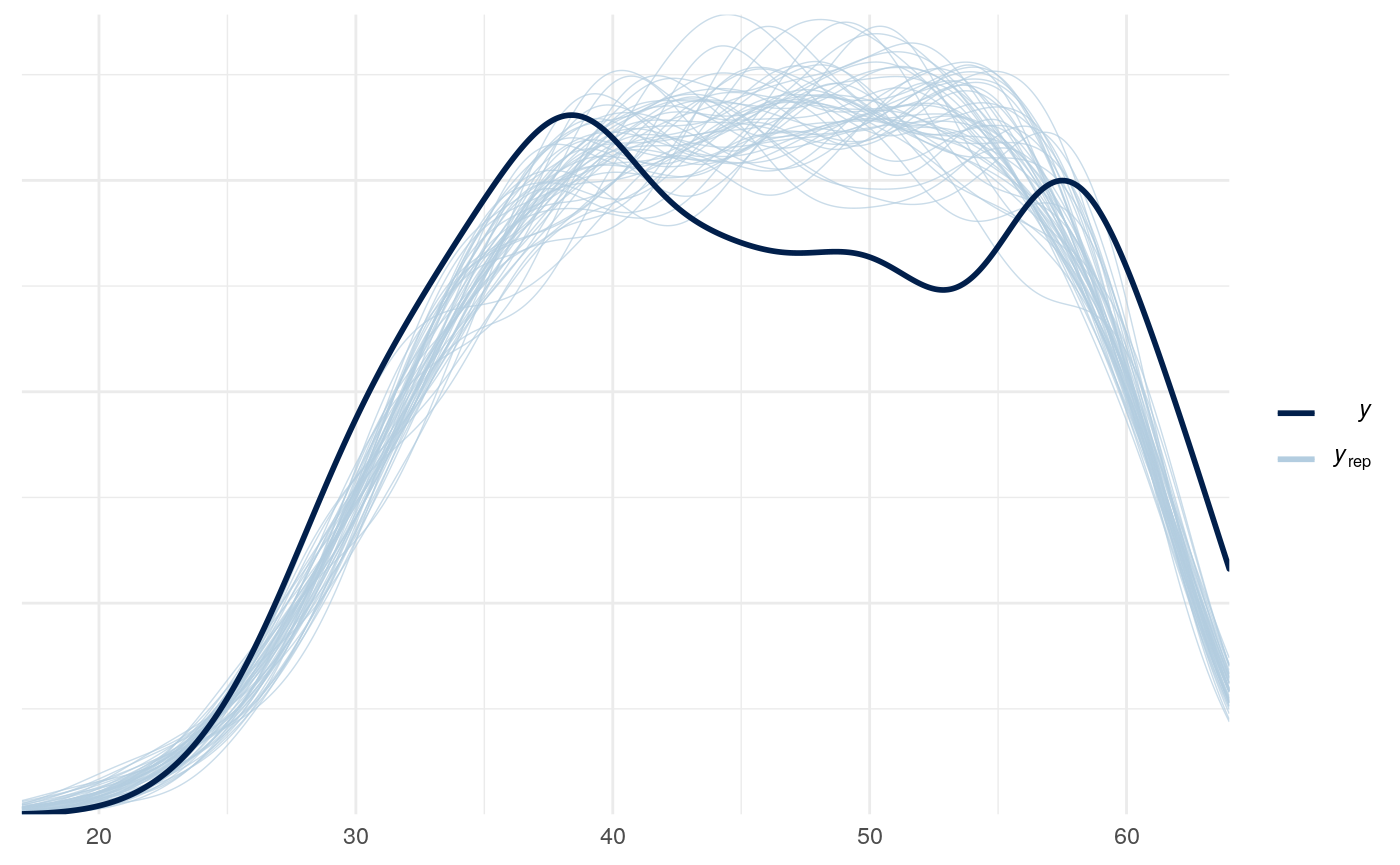
One thing that is obvious from the posterior predictive check of this model is that there is more going on than a simple bernoulli process. The distribution of y values is lumpy and bi-modal in a way that suggests a mixture of probabilities of success in the latter trials. Conditioning on word-pairs, age, and self report questionnairs does not help explain these differences.
Results from logistic regression
#> [1] FALSE
#> Generalized linear mixed model fit by maximum likelihood (Laplace
#>   Approximation) [glmerMod]
#>  Family: binomial  ( logit )
#> Formula: press_opt ~ 1 + (1 | id)
#>    Data: splt
#>
#>      AIC      BIC   logLik deviance df.resid
#> 141034.9 141054.3 -70515.5 141030.9   116704
#>
#> Scaled residuals:
#>     Min      1Q  Median      3Q     Max
#> -3.2363 -1.1166  0.5409  0.7263  1.0859
#>
#> Random effects:
#>  Groups Name        Variance Std.Dev.
#>  id     (Intercept) 0.2929   0.5412
#> Number of obs: 116706, groups:  id, 308
#>
#> Fixed effects:
#>             Estimate Std. Error z value Pr(>|z|)
#> (Intercept)  0.79811    0.03149   25.35   <2e-16 ***
#> ---
#> Signif. codes:  0 '***' 0.001 '**' 0.01 '*' 0.05 '.' 0.1 ' ' 1
#> Generalized linear mixed model fit by maximum likelihood (Laplace
#>   Approximation) [glmerMod]
#>  Family: binomial  ( logit )
#> Formula: press_opt ~ 1 + (1 | sample/id)
#>    Data: splt
#>
#>      AIC      BIC   logLik deviance df.resid
#> 141024.6 141053.6 -70509.3 141018.6   116703
#>
#> Scaled residuals:
#>     Min      1Q  Median      3Q     Max
#> -3.2523 -1.1174  0.5386  0.7274  1.0865
#>
#> Random effects:
#>  Groups    Name        Variance Std.Dev.
#>  id:sample (Intercept) 0.27371  0.5232
#>  sample    (Intercept) 0.02302  0.1517
#> Number of obs: 116706, groups:  id:sample, 308; sample, 4
#>
#> Fixed effects:
#>             Estimate Std. Error z value Pr(>|z|)
#> (Intercept)  0.78396    0.08295   9.451   <2e-16 ***
#> ---
#> Signif. codes:  0 '***' 0.001 '**' 0.01 '*' 0.05 '.' 0.1 ' ' 1
#> Generalized linear mixed model fit by maximum likelihood (Laplace
#>   Approximation) [glmerMod]
#>  Family: binomial  ( logit )
#> Formula: press_opt ~ 1 + (1 | sample/id) + (1 | stim_image)
#>    Data: splt
#>
#>      AIC      BIC   logLik deviance df.resid
#> 140572.2 140610.8 -70282.1 140564.2   116702
#>
#> Scaled residuals:
#>     Min      1Q  Median      3Q     Max
#> -3.5014 -1.1146  0.5343  0.7173  1.2401
#>
#> Random effects:
#>  Groups     Name        Variance Std.Dev.
#>  id:sample  (Intercept) 0.27594  0.5253
#>  stim_image (Intercept) 0.02193  0.1481
#>  sample     (Intercept) 0.02588  0.1609
#> Number of obs: 116706, groups:  id:sample, 308; stim_image, 6; sample, 4
#>
#> Fixed effects:
#>             Estimate Std. Error z value Pr(>|z|)
#> (Intercept)   0.7862     0.1060   7.416 1.21e-13 ***
#> ---
#> Signif. codes:  0 '***' 0.001 '**' 0.01 '*' 0.05 '.' 0.1 ' ' 1
#> (Intercept)
#>   0.6895691
#> (Intercept)
#>   0.6865322
#> (Intercept)
#> 0.687019| npar | AIC | BIC | logLik | deviance | Chisq | Df | Pr(>Chisq) | |
|---|---|---|---|---|---|---|---|---|
| check_stim_rx_null_id_only_m | 2 | 141034.9 | 141054.3 | -70515.47 | 141030.9 | |||
| check_stim_rx_null_m | 3 | 141024.6 | 141053.6 | -70509.32 | 141018.6 | 12.3136 | 1 | 4e-04 |
| check_stim_rx_null_stim_rx_m | 4 | 140572.2 | 140610.8 | -70282.08 | 140564.2 | 454.4771 | 1 | 0e+00 |
| npar | AIC | BIC | logLik | deviance | Chisq | Df | Pr(>Chisq) | |
|---|---|---|---|---|---|---|---|---|
| null_lm | 4 | 140572.2 | 140610.8 | -70282.08 | 140564.2 | |||
| time_lm | 9 | 137966.5 | 138053.5 | -68974.27 | 137948.5 | 2615.626 | 5 | 0 |
| npar | AIC | BIC | logLik | deviance | Chisq | Df | Pr(>Chisq) | |
|---|---|---|---|---|---|---|---|---|
| null_lm | 4 | 140572.2 | 140610.8 | -70282.08 | 140564.2 | |||
| condition_lm | 16 | 139442.8 | 139597.5 | -69705.39 | 139410.8 | 1153.378 | 12 | 0 |
#> Generalized linear mixed model fit by maximum likelihood (Laplace
#> Approximation) [glmerMod]
#> Family: binomial ( logit )
#> Formula: press_opt ~ 1 + condition * trial_index_c0_s * age_std * gender +
#> (1 + condition * trial_index_c0_s | sample:id)
#> Data: splt
#> Control: lme4_control_options
#>
#> AIC BIC logLik deviance df.resid
#> 137130.5 137565.6 -68520.3 137040.5 116661
#>
#> Scaled residuals:
#> Min 1Q Median 3Q Max
#> -7.2937 -1.0555 0.4768 0.7451 1.6287
#>
#> Random effects:
#> Groups Name Variance Std.Dev. Corr
#> sample:id (Intercept) 1.39053 1.1792
#> conditionDating/Looking 0.75153 0.8669 -0.25
#> conditionPopular/Unpopular 0.52033 0.7213 -0.18
#> trial_index_c0_s 0.09669 0.3110 0.96
#> conditionDating/Looking:trial_index_c0_s 0.07520 0.2742 -0.10
#> conditionPopular/Unpopular:trial_index_c0_s 0.05383 0.2320 -0.06
#>
#>
#>
#> 0.45
#> -0.16 0.10
#> 0.79 0.24 -0.06
#> 0.36 0.64 0.13 0.41
#> Number of obs: 116706, groups: sample:id, 308
#>
#> Fixed effects:
#> Estimate
#> (Intercept) 1.0226875
#> conditionDating/Looking 0.1414945
#> conditionPopular/Unpopular 0.2189603
#> trial_index_c0_s 0.2303013
#> age_std 0.0762011
#> genderFemale 0.3248039
#> conditionDating/Looking:trial_index_c0_s -0.0028288
#> conditionPopular/Unpopular:trial_index_c0_s 0.0059656
#> conditionDating/Looking:age_std -0.0135116
#> conditionPopular/Unpopular:age_std -0.0052754
#> trial_index_c0_s:age_std 0.0130405
#> conditionDating/Looking:genderFemale -0.0149832
#> conditionPopular/Unpopular:genderFemale -0.0308998
#> trial_index_c0_s:genderFemale 0.0568792
#> age_std:genderFemale 0.0238716
#> conditionDating/Looking:trial_index_c0_s:age_std -0.0192557
#> conditionPopular/Unpopular:trial_index_c0_s:age_std -0.0115440
#> conditionDating/Looking:trial_index_c0_s:genderFemale 0.0075287
#> conditionPopular/Unpopular:trial_index_c0_s:genderFemale 0.0135768
#> conditionDating/Looking:age_std:genderFemale -0.1243677
#> conditionPopular/Unpopular:age_std:genderFemale 0.0321801
#> trial_index_c0_s:age_std:genderFemale 0.0000271
#> conditionDating/Looking:trial_index_c0_s:age_std:genderFemale -0.0260058
#> conditionPopular/Unpopular:trial_index_c0_s:age_std:genderFemale 0.0398148
#> Std. Error
#> (Intercept) 0.1220392
#> conditionDating/Looking 0.1033806
#> conditionPopular/Unpopular 0.0918774
#> trial_index_c0_s 0.0359863
#> age_std 0.1030089
#> genderFemale 0.1506542
#> conditionDating/Looking:trial_index_c0_s 0.0388166
#> conditionPopular/Unpopular:trial_index_c0_s 0.0360532
#> conditionDating/Looking:age_std 0.0863625
#> conditionPopular/Unpopular:age_std 0.0762590
#> trial_index_c0_s:age_std 0.0303211
#> conditionDating/Looking:genderFemale 0.1277171
#> conditionPopular/Unpopular:genderFemale 0.1131608
#> trial_index_c0_s:genderFemale 0.0444625
#> age_std:genderFemale 0.1429447
#> conditionDating/Looking:trial_index_c0_s:age_std 0.0324309
#> conditionPopular/Unpopular:trial_index_c0_s:age_std 0.0299334
#> conditionDating/Looking:trial_index_c0_s:genderFemale 0.0479496
#> conditionPopular/Unpopular:trial_index_c0_s:genderFemale 0.0444028
#> conditionDating/Looking:age_std:genderFemale 0.1210167
#> conditionPopular/Unpopular:age_std:genderFemale 0.1066808
#> trial_index_c0_s:age_std:genderFemale 0.0421695
#> conditionDating/Looking:trial_index_c0_s:age_std:genderFemale 0.0454347
#> conditionPopular/Unpopular:trial_index_c0_s:age_std:genderFemale 0.0418571
#> z value
#> (Intercept) 8.380
#> conditionDating/Looking 1.369
#> conditionPopular/Unpopular 2.383
#> trial_index_c0_s 6.400
#> age_std 0.740
#> genderFemale 2.156
#> conditionDating/Looking:trial_index_c0_s -0.073
#> conditionPopular/Unpopular:trial_index_c0_s 0.165
#> conditionDating/Looking:age_std -0.156
#> conditionPopular/Unpopular:age_std -0.069
#> trial_index_c0_s:age_std 0.430
#> conditionDating/Looking:genderFemale -0.117
#> conditionPopular/Unpopular:genderFemale -0.273
#> trial_index_c0_s:genderFemale 1.279
#> age_std:genderFemale 0.167
#> conditionDating/Looking:trial_index_c0_s:age_std -0.594
#> conditionPopular/Unpopular:trial_index_c0_s:age_std -0.386
#> conditionDating/Looking:trial_index_c0_s:genderFemale 0.157
#> conditionPopular/Unpopular:trial_index_c0_s:genderFemale 0.306
#> conditionDating/Looking:age_std:genderFemale -1.028
#> conditionPopular/Unpopular:age_std:genderFemale 0.302
#> trial_index_c0_s:age_std:genderFemale 0.001
#> conditionDating/Looking:trial_index_c0_s:age_std:genderFemale -0.572
#> conditionPopular/Unpopular:trial_index_c0_s:age_std:genderFemale 0.951
#> Pr(>|z|)
#> (Intercept) < 2e-16 ***
#> conditionDating/Looking 0.1711
#> conditionPopular/Unpopular 0.0172 *
#> trial_index_c0_s 1.56e-10 ***
#> age_std 0.4595
#> genderFemale 0.0311 *
#> conditionDating/Looking:trial_index_c0_s 0.9419
#> conditionPopular/Unpopular:trial_index_c0_s 0.8686
#> conditionDating/Looking:age_std 0.8757
#> conditionPopular/Unpopular:age_std 0.9448
#> trial_index_c0_s:age_std 0.6671
#> conditionDating/Looking:genderFemale 0.9066
#> conditionPopular/Unpopular:genderFemale 0.7848
#> trial_index_c0_s:genderFemale 0.2008
#> age_std:genderFemale 0.8674
#> conditionDating/Looking:trial_index_c0_s:age_std 0.5527
#> conditionPopular/Unpopular:trial_index_c0_s:age_std 0.6998
#> conditionDating/Looking:trial_index_c0_s:genderFemale 0.8752
#> conditionPopular/Unpopular:trial_index_c0_s:genderFemale 0.7598
#> conditionDating/Looking:age_std:genderFemale 0.3041
#> conditionPopular/Unpopular:age_std:genderFemale 0.7629
#> trial_index_c0_s:age_std:genderFemale 0.9995
#> conditionDating/Looking:trial_index_c0_s:age_std:genderFemale 0.5671
#> conditionPopular/Unpopular:trial_index_c0_s:age_std:genderFemale 0.3415
#> ---
#> Signif. codes: 0 '***' 0.001 '**' 0.01 '*' 0.05 '.' 0.1 ' ' 1
#> convergence code: 0
#> unable to evaluate scaled gradient
#> Model failed to converge: degenerate Hessian with 1 negative eigenvalues
#> Generalized linear mixed model fit by maximum likelihood (Laplace
#> Approximation) [glmerMod]
#> Family: binomial ( logit )
#> Formula: press_opt ~ 1 + condition * trial_index_c0_s * pds_std * gender +
#> (1 + condition * trial_index_c0_s | sample:id)
#> Data: splt
#> Control: lme4_control_options
#>
#> AIC BIC logLik deviance df.resid
#> 134325.1 134759.1 -67117.6 134235.1 114009
#>
#> Scaled residuals:
#> Min 1Q Median 3Q Max
#> -7.0046 -1.0562 0.4788 0.7490 1.6757
#>
#> Random effects:
#> Groups Name Variance Std.Dev. Corr
#> sample:id (Intercept) 1.32345 1.1504
#> conditionDating/Looking 0.66107 0.8131 -0.18
#> conditionPopular/Unpopular 0.55681 0.7462 -0.16
#> trial_index_c0_s 0.08921 0.2987 0.96
#> conditionDating/Looking:trial_index_c0_s 0.06670 0.2583 -0.03
#> conditionPopular/Unpopular:trial_index_c0_s 0.05590 0.2364 -0.02
#>
#>
#>
#> 0.37
#> -0.02 0.12
#> 0.74 0.18 0.07
#> 0.21 0.67 0.17 0.30
#> Number of obs: 114054, groups: sample:id, 301
#>
#> Fixed effects:
#> Estimate
#> (Intercept) 1.104414
#> conditionDating/Looking 0.097405
#> conditionPopular/Unpopular 0.187511
#> trial_index_c0_s 0.253568
#> pds_std 0.136736
#> genderFemale 0.155509
#> conditionDating/Looking:trial_index_c0_s -0.029583
#> conditionPopular/Unpopular:trial_index_c0_s -0.022551
#> conditionDating/Looking:pds_std -0.072509
#> conditionPopular/Unpopular:pds_std -0.039470
#> trial_index_c0_s:pds_std 0.037576
#> conditionDating/Looking:genderFemale 0.097438
#> conditionPopular/Unpopular:genderFemale -0.009530
#> trial_index_c0_s:genderFemale 0.006425
#> pds_std:genderFemale 0.021213
#> conditionDating/Looking:trial_index_c0_s:pds_std -0.045289
#> conditionPopular/Unpopular:trial_index_c0_s:pds_std -0.042435
#> conditionDating/Looking:trial_index_c0_s:genderFemale 0.048857
#> conditionPopular/Unpopular:trial_index_c0_s:genderFemale 0.046768
#> conditionDating/Looking:pds_std:genderFemale -0.022967
#> conditionPopular/Unpopular:pds_std:genderFemale 0.157159
#> trial_index_c0_s:pds_std:genderFemale 0.013477
#> conditionDating/Looking:trial_index_c0_s:pds_std:genderFemale 0.038699
#> conditionPopular/Unpopular:trial_index_c0_s:pds_std:genderFemale 0.067117
#> Std. Error
#> (Intercept) 0.132499
#> conditionDating/Looking 0.109697
#> conditionPopular/Unpopular 0.104208
#> trial_index_c0_s 0.038823
#> pds_std 0.097320
#> genderFemale 0.163291
#> conditionDating/Looking:trial_index_c0_s 0.041826
#> conditionPopular/Unpopular:trial_index_c0_s 0.040411
#> conditionDating/Looking:pds_std 0.079442
#> conditionPopular/Unpopular:pds_std 0.075042
#> trial_index_c0_s:pds_std 0.028378
#> conditionDating/Looking:genderFemale 0.135365
#> conditionPopular/Unpopular:genderFemale 0.127750
#> trial_index_c0_s:genderFemale 0.047843
#> pds_std:genderFemale 0.160721
#> conditionDating/Looking:trial_index_c0_s:pds_std 0.030220
#> conditionPopular/Unpopular:trial_index_c0_s:pds_std 0.029034
#> conditionDating/Looking:trial_index_c0_s:genderFemale 0.051600
#> conditionPopular/Unpopular:trial_index_c0_s:genderFemale 0.049523
#> conditionDating/Looking:pds_std:genderFemale 0.132350
#> conditionPopular/Unpopular:pds_std:genderFemale 0.124484
#> trial_index_c0_s:pds_std:genderFemale 0.046920
#> conditionDating/Looking:trial_index_c0_s:pds_std:genderFemale 0.050356
#> conditionPopular/Unpopular:trial_index_c0_s:pds_std:genderFemale 0.048122
#> z value
#> (Intercept) 8.335
#> conditionDating/Looking 0.888
#> conditionPopular/Unpopular 1.799
#> trial_index_c0_s 6.531
#> pds_std 1.405
#> genderFemale 0.952
#> conditionDating/Looking:trial_index_c0_s -0.707
#> conditionPopular/Unpopular:trial_index_c0_s -0.558
#> conditionDating/Looking:pds_std -0.913
#> conditionPopular/Unpopular:pds_std -0.526
#> trial_index_c0_s:pds_std 1.324
#> conditionDating/Looking:genderFemale 0.720
#> conditionPopular/Unpopular:genderFemale -0.075
#> trial_index_c0_s:genderFemale 0.134
#> pds_std:genderFemale 0.132
#> conditionDating/Looking:trial_index_c0_s:pds_std -1.499
#> conditionPopular/Unpopular:trial_index_c0_s:pds_std -1.462
#> conditionDating/Looking:trial_index_c0_s:genderFemale 0.947
#> conditionPopular/Unpopular:trial_index_c0_s:genderFemale 0.944
#> conditionDating/Looking:pds_std:genderFemale -0.174
#> conditionPopular/Unpopular:pds_std:genderFemale 1.262
#> trial_index_c0_s:pds_std:genderFemale 0.287
#> conditionDating/Looking:trial_index_c0_s:pds_std:genderFemale 0.769
#> conditionPopular/Unpopular:trial_index_c0_s:pds_std:genderFemale 1.395
#> Pr(>|z|)
#> (Intercept) < 2e-16 ***
#> conditionDating/Looking 0.375
#> conditionPopular/Unpopular 0.072 .
#> trial_index_c0_s 6.52e-11 ***
#> pds_std 0.160
#> genderFemale 0.341
#> conditionDating/Looking:trial_index_c0_s 0.479
#> conditionPopular/Unpopular:trial_index_c0_s 0.577
#> conditionDating/Looking:pds_std 0.361
#> conditionPopular/Unpopular:pds_std 0.599
#> trial_index_c0_s:pds_std 0.185
#> conditionDating/Looking:genderFemale 0.472
#> conditionPopular/Unpopular:genderFemale 0.941
#> trial_index_c0_s:genderFemale 0.893
#> pds_std:genderFemale 0.895
#> conditionDating/Looking:trial_index_c0_s:pds_std 0.134
#> conditionPopular/Unpopular:trial_index_c0_s:pds_std 0.144
#> conditionDating/Looking:trial_index_c0_s:genderFemale 0.344
#> conditionPopular/Unpopular:trial_index_c0_s:genderFemale 0.345
#> conditionDating/Looking:pds_std:genderFemale 0.862
#> conditionPopular/Unpopular:pds_std:genderFemale 0.207
#> trial_index_c0_s:pds_std:genderFemale 0.774
#> conditionDating/Looking:trial_index_c0_s:pds_std:genderFemale 0.442
#> conditionPopular/Unpopular:trial_index_c0_s:pds_std:genderFemale 0.163
#> ---
#> Signif. codes: 0 '***' 0.001 '**' 0.01 '*' 0.05 '.' 0.1 ' ' 1
#> convergence code: 0
#> unable to evaluate scaled gradient
#> Model failed to converge: degenerate Hessian with 1 negative eigenvalues
#> Generalized linear mixed model fit by maximum likelihood (Laplace
#> Approximation) [glmerMod]
#> Family: binomial ( logit )
#> Formula: press_opt ~ 1 + condition * condition_trial_index_c0_s + (condition *
#> condition_trial_index_c0_s | id)
#> Data: splt
#>
#> AIC BIC logLik deviance df.resid
#> 136881.0 137142.0 -68413.5 136827.0 116679
#>
#> Scaled residuals:
#> Min 1Q Median 3Q Max
#> -7.1848 -1.0469 0.4738 0.7424 1.6666
#>
#> Random effects:
#> Groups Name Variance Std.Dev.
#> id (Intercept) 1.6930 1.3012
#> conditionDating/Looking 0.9194 0.9589
#> conditionPopular/Unpopular 0.9884 0.9942
#> condition_trial_index_c0_s 0.1688 0.4108
#> conditionDating/Looking:condition_trial_index_c0_s 0.1123 0.3351
#> conditionPopular/Unpopular:condition_trial_index_c0_s 0.1311 0.3621
#> Corr
#>
#> -0.38
#> -0.38 0.58
#> 0.92 -0.39 -0.37
#> -0.31 0.83 0.54 -0.42
#> -0.32 0.53 0.83 -0.44 0.65
#> Number of obs: 116706, groups: id, 308
#>
#> Fixed effects:
#> Estimate Std. Error
#> (Intercept) 1.267727 0.078911
#> conditionDating/Looking 0.100667 0.066840
#> conditionPopular/Unpopular 0.179051 0.068698
#> condition_trial_index_c0_s 0.277563 0.026488
#> conditionDating/Looking:condition_trial_index_c0_s -0.007297 0.026020
#> conditionPopular/Unpopular:condition_trial_index_c0_s 0.009664 0.027233
#> z value Pr(>|z|)
#> (Intercept) 16.065 < 2e-16 ***
#> conditionDating/Looking 1.506 0.13204
#> conditionPopular/Unpopular 2.606 0.00915 **
#> condition_trial_index_c0_s 10.479 < 2e-16 ***
#> conditionDating/Looking:condition_trial_index_c0_s -0.280 0.77915
#> conditionPopular/Unpopular:condition_trial_index_c0_s 0.355 0.72268
#> ---
#> Signif. codes: 0 '***' 0.001 '**' 0.01 '*' 0.05 '.' 0.1 ' ' 1
#>
#> Correlation of Fixed Effects:
#> (Intr) cndD/L cndP/U c___0_ cD/L:_
#> cndtnDtng/L -0.433
#> cndtnPplr/U -0.429 0.551
#> cndtn_t__0_ 0.905 -0.448 -0.436
#> cnD/L:___0_ -0.359 0.848 0.495 -0.497
#> cnP/U:___0_ -0.369 0.493 0.849 -0.508 0.577
#> convergence code: 0
#> Model failed to converge with max|grad| = 0.0432773 (tol = 0.001, component 1)
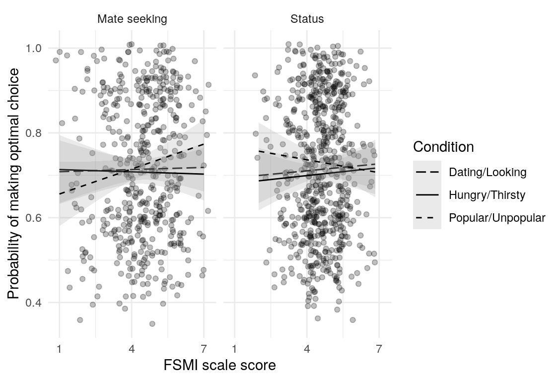
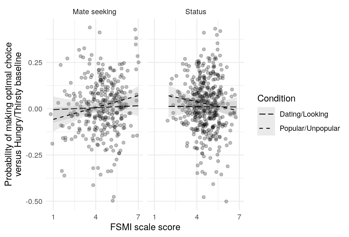
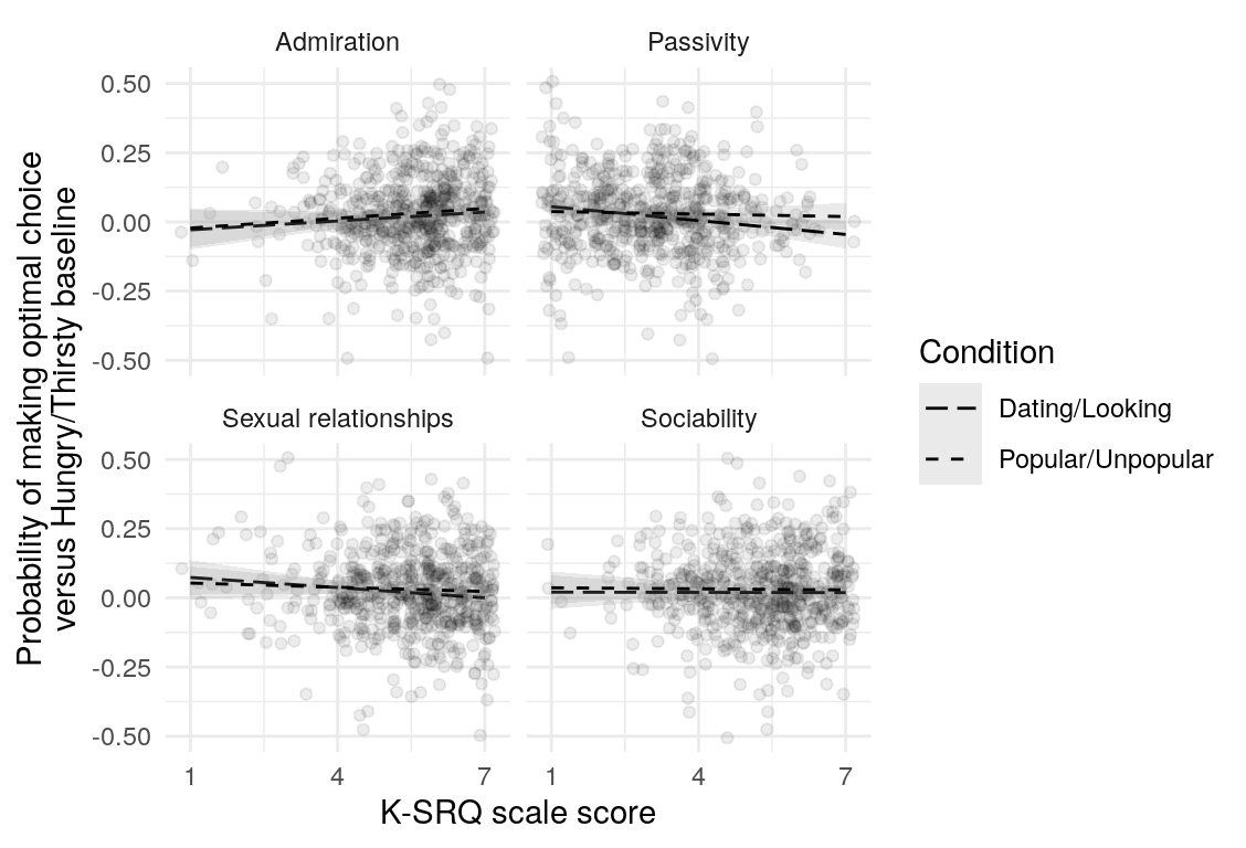
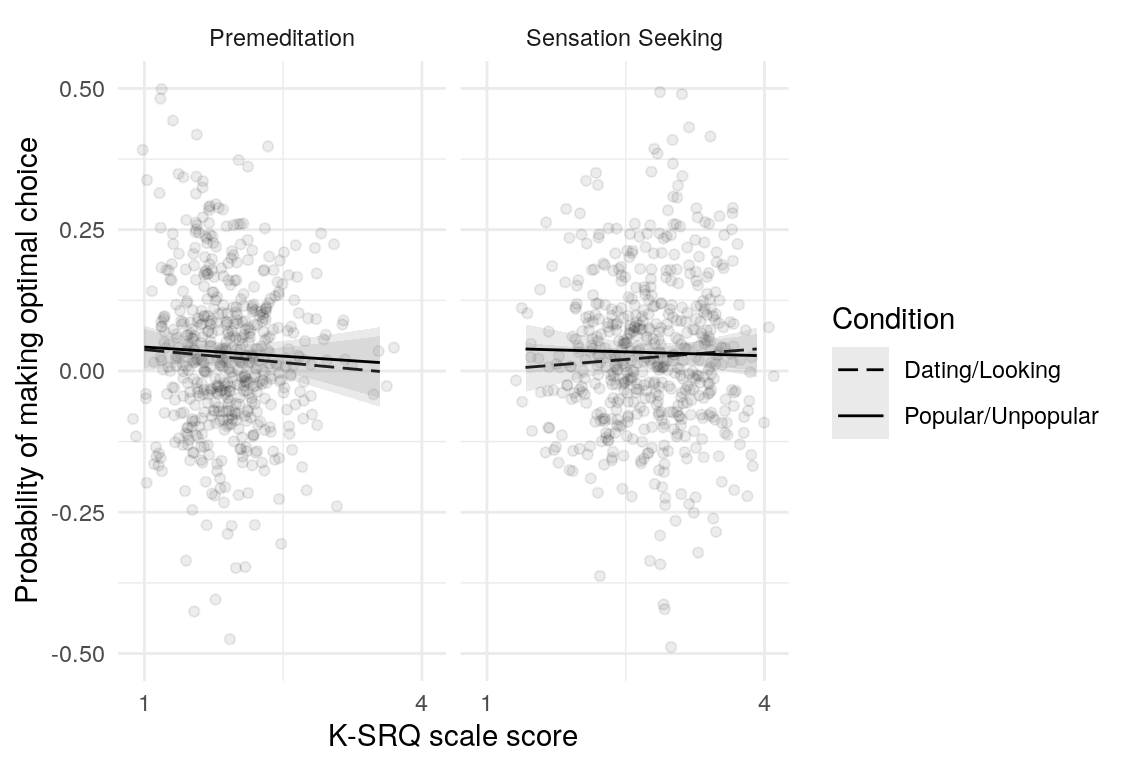
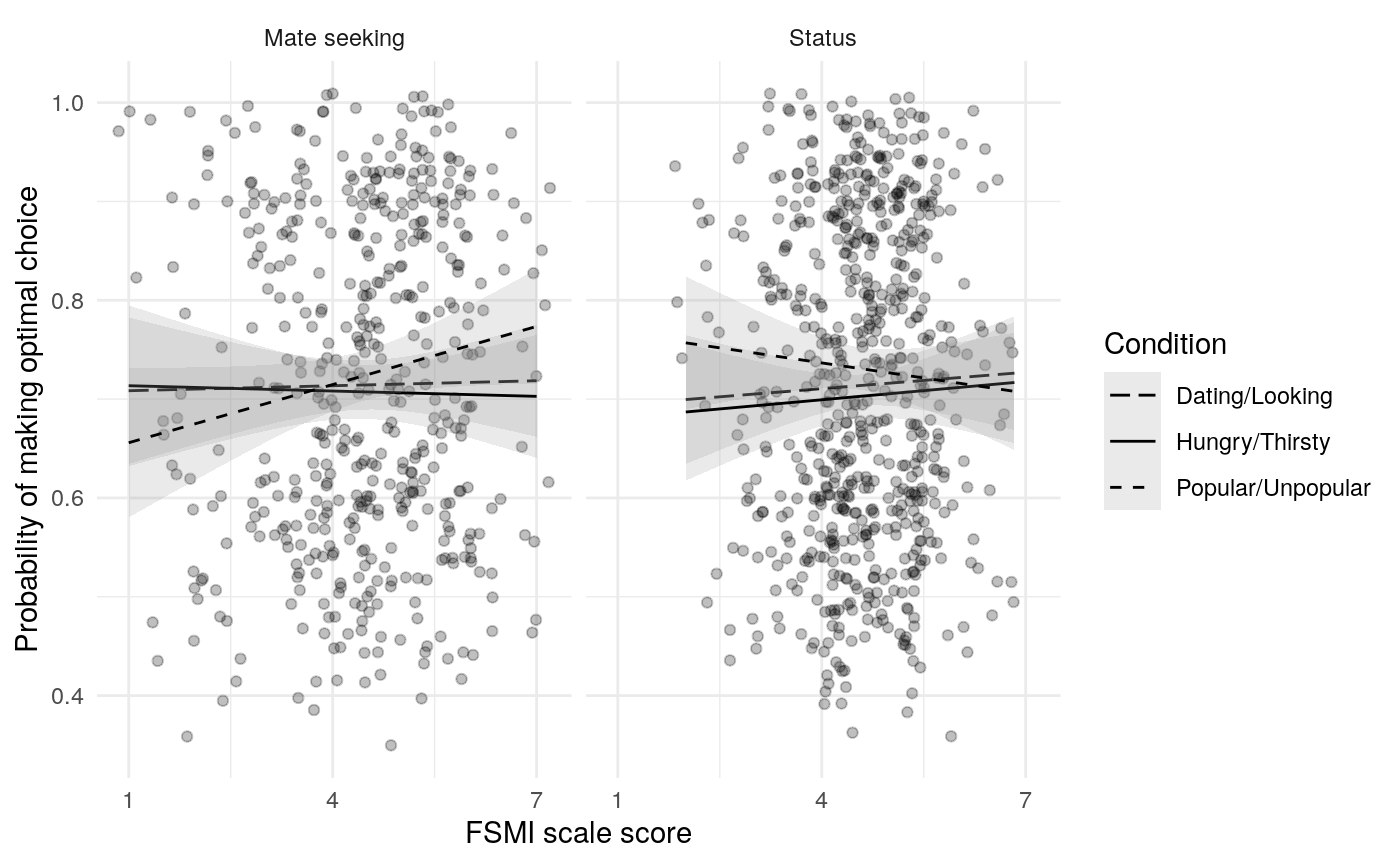
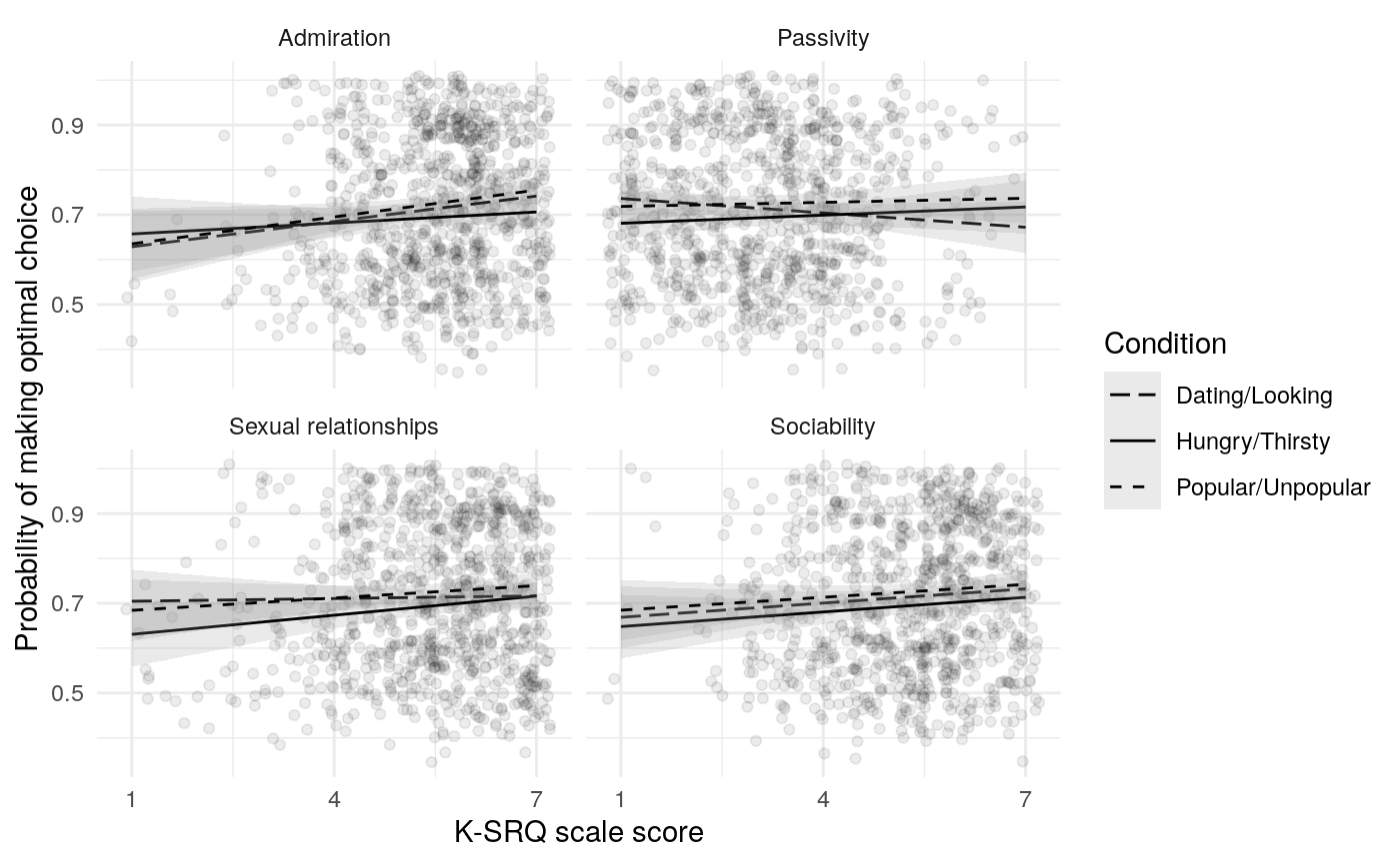
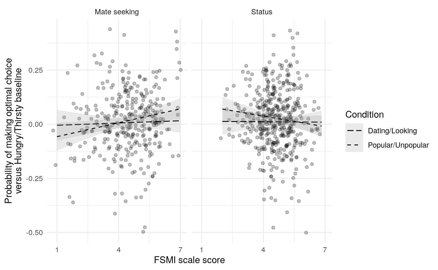
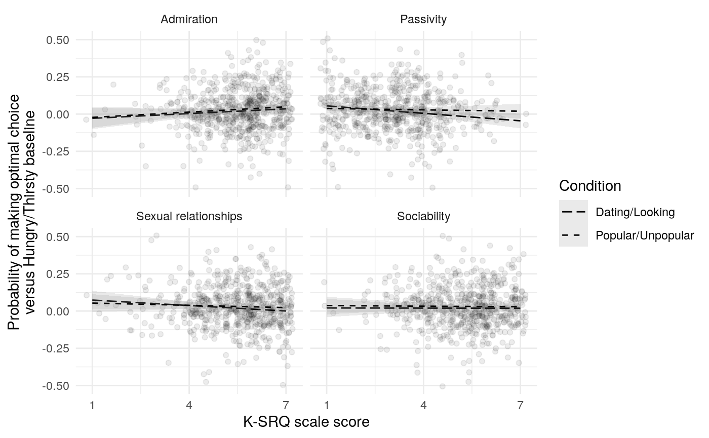
#> [1] 0.24520291 0.13315981 0.14315331 0.02444787 0.01626479 0.01898766Relation to FSMI subscales
| Scale | \(\omega_h\) | \(\omega_t\) | \(\alpha\) |
|---|---|---|---|
| FSMI mate-seeking | 0.88 | 0.89 | 0.88 |
| FSMI status | 0.72 | 0.72 | 0.71 |
| K-SRQ sexual relationships factor | —- | —- | 0.77 |
| K-SRQ admiration factor | —- | —- | 0.86 |
| K-SRQ sexual relationships scale | —- | —- | 0.76 |
| K-SRQ admiration scale | —- | —- | 0.86 |
| Dominance | 0.63 | 0.87 | 0.83 |
| Prestige | 0.57 | 0.86 | 0.81 |
| Sensation seeking | 0.59 | 0.87 | 0.81 |
In addition to confirmatory factor analyses, scale reliability and general-factor validity were assessed via the \(\omega_{h}\) and \(\omega_t\) statistics. These statistics account for the possibility that variance on items is due to both a general latent factor common to all items, and several group fators that account for variance in subsets of items (Zinbarg, Yovel, Revelle, & McDonald, 2006). The \(\omega_{h}\) statistic captures the proportion of variance due to a general factor, and so is proportional to the degree of expected correspondence between the scale and another measure of the construct (on a different scale, or at retest), and also indexes the validity of the scale as a measure of the ostensible latent construct. The reliability of the whole scale is indexed by \(\omega_t\), which includes variance due to both group and general factors. Cronebach’s \(\alpha\) is also reported because it is the default practice, and it may be helpful to demonstrate the differences between the two approaches. All three statistics were calculated using the omega function in the psych package for R (Revelle, 2017).
The mate-seeking and status motive scales from the FSMI showed adequate reliability, with \(\alpha\) and \(\omega_t\) in the acceptable to excellent range according to some rules of thumb (Table ref(tab:fsmi_reliability). However, \(\omega_h\) indicates that only about 68% of the variance in FSMI Status and 80% of the variance in FSMI mate-seeking are due to the general factor. In light of this, any correlations of scale responses with other constructs of interest should be interpretted in light of the possibility that they are due, in part, to associations between variance not due to the general factor (and thus note due to the construct of interest). Of course, the variance due to other latent causes may also be a reason true relations are attentuated.
Results from Bayesian learning models
Model comparison
Models labeled “repar_exp” are 3-level models, whereas those labeled “2_level” are 2-level models.
| elpd_diff | se_diff | elpd_loo | se_elpd_loo | p_loo | se_p_loo | looic | se_looic | |
|---|---|---|---|---|---|---|---|---|
| splt-looser-rl_2_level-1545567.RDS | 0.00000 | 0.00000 | -67279.32 | 749.8435 | 1324.9518 | 25.93839 | 134558.6 | 1499.687 |
| splt-looser-rl_repar_exp-1528144.RDS | -15.03629 | 10.95402 | -67294.35 | 748.7886 | 1336.3750 | 26.51125 | 134588.7 | 1497.577 |
| splt-looser-rl_repar_exp_no_b-1528233.RDS | -661.45148 | 65.33014 | -67940.77 | 749.0423 | 932.6000 | 24.77321 | 135881.5 | 1498.085 |
| splt-looser-rl_2_level_no_b-1527784.RDS | -666.88784 | 65.19907 | -67946.20 | 748.9929 | 937.6198 | 24.46348 | 135892.4 | 1497.986 |
| splt-looser-rl_repar_exp_no_b_no_rho-1527735.RDS | -1166.03330 | 89.83720 | -68445.35 | 703.3801 | 736.0842 | 20.12318 | 136890.7 | 1406.760 |
| splt-looser-rl_2_level_no_b_no_rho-1527729.RDS | -1178.27166 | 89.38079 | -68457.59 | 703.2658 | 746.3897 | 19.63269 | 136915.2 | 1406.532 |
If we can trust these LOO estimates (it would be better to do leave-one-observation-out rather than leave-one-participant-out), it looks like the three level structure is probably unnecessary but that the full parameterization is helpful.
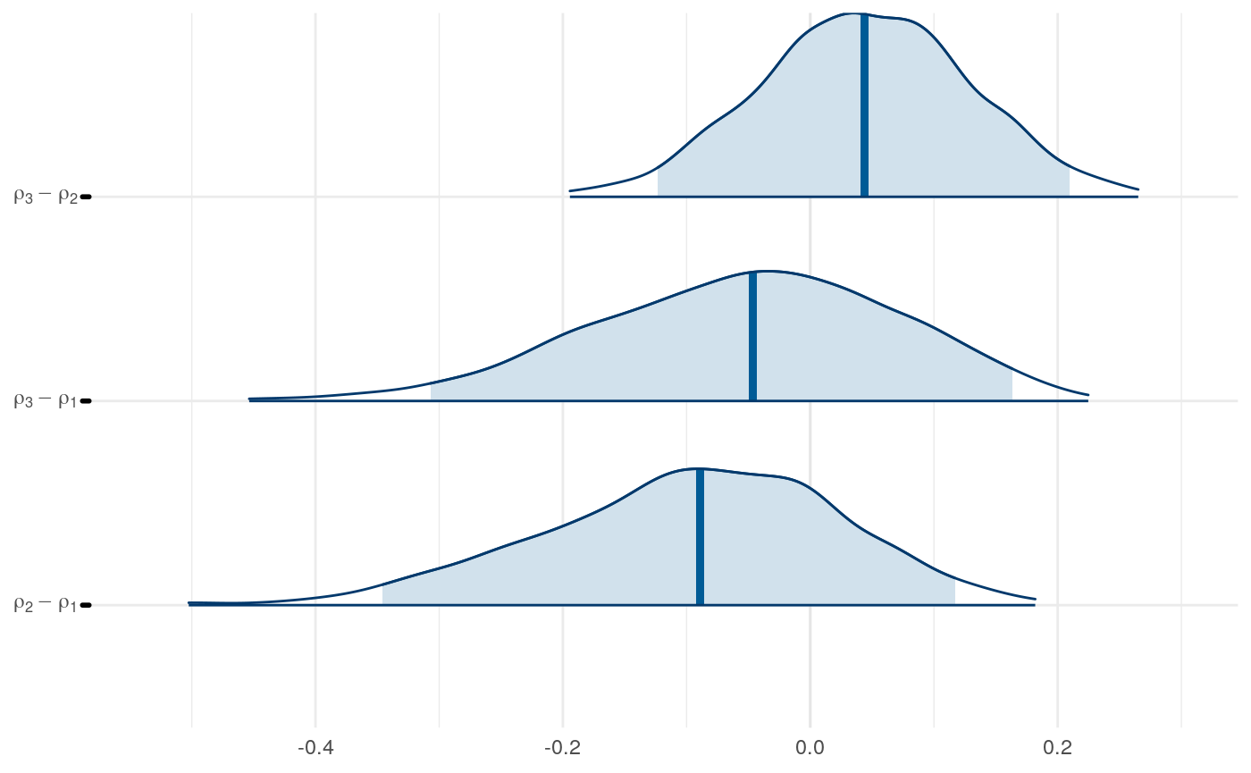
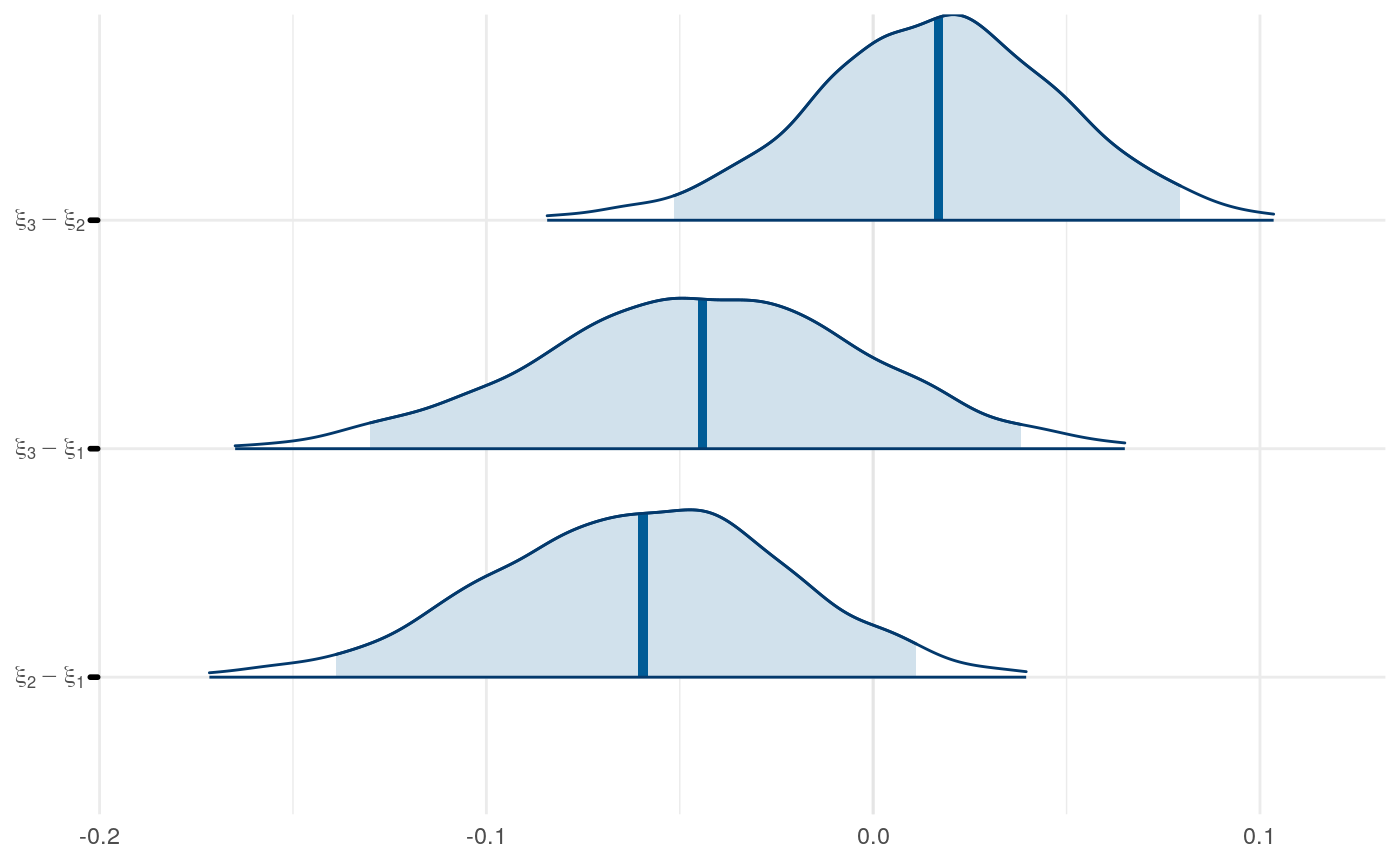
We can examine differences in some of the parameters across models to get a sense for this as well.
We can also examine the correlation of parameters as we drop the terms \(b\) and \(\rho\) from the continuous-\(\rho\) models.
#> Call:psych::corr.test(x = dplyr::select(par_means_for_corplot, contains("eps")))
#> Correlation matrix
#>                      epsilon["max"] epsilon["no b"] epsilon["no b,"~rho]
#> epsilon["max"]                 1.00            0.92                 0.84
#> epsilon["no b"]                0.92            1.00                 0.90
#> epsilon["no b,"~rho]           0.84            0.90                 1.00
#> Sample Size
#> [1] 939
#> Probability values (Entries above the diagonal are adjusted for multiple tests.)
#>                      epsilon["max"] epsilon["no b"] epsilon["no b,"~rho]
#> epsilon["max"]                    0               0                    0
#> epsilon["no b"]                   0               0                    0
#> epsilon["no b,"~rho]              0               0                    0
#>
#>  To see confidence intervals of the correlations, print with the short=FALSE option
#> Call:psych::corr.test(x = dplyr::select(par_means_for_corplot, contains("xi")))
#> Correlation matrix
#>                 xi["max"] xi["no b"] xi["no b,"~rho]
#> xi["max"]            1.00       0.93            0.88
#> xi["no b"]           0.93       1.00            0.96
#> xi["no b,"~rho]      0.88       0.96            1.00
#> Sample Size
#> [1] 939
#> Probability values (Entries above the diagonal are adjusted for multiple tests.)
#>                 xi["max"] xi["no b"] xi["no b,"~rho]
#> xi["max"]               0          0               0
#> xi["no b"]              0          0               0
#> xi["no b,"~rho]         0          0               0
#>
#>  To see confidence intervals of the correlations, print with the short=FALSE option
#> Call:psych::corr.test(x = dplyr::select(par_means_for_corplot, contains("rho[")))
#> Correlation matrix
#>             rho["max"] rho["no b"]
#> rho["max"]        1.00        0.68
#> rho["no b"]       0.68        1.00
#> Sample Size
#> [1] 939
#> Probability values (Entries above the diagonal are adjusted for multiple tests.)
#>             rho["max"] rho["no b"]
#> rho["max"]           0           0
#> rho["no b"]          0           0
#>
#>  To see confidence intervals of the correlations, print with the short=FALSE option
#> Call:psych::corr.test(x = dplyr::select(par_means_for_corplot, contains("max")),
#>     method = "spearman")
#> Correlation matrix
#>                epsilon["max"] xi["max"] rho["max"] b["max"]
#> epsilon["max"]           1.00      0.19      -0.17    -0.04
#> xi["max"]                0.19      1.00      -0.34     0.03
#> rho["max"]              -0.17     -0.34       1.00     0.10
#> b["max"]                -0.04      0.03       0.10     1.00
#> Sample Size
#> [1] 939
#> Probability values (Entries above the diagonal are adjusted for multiple tests.)
#>                epsilon["max"] xi["max"] rho["max"] b["max"]
#> epsilon["max"]           0.00      0.00          0     0.52
#> xi["max"]                0.00      0.00          0     0.52
#> rho["max"]               0.00      0.00          0     0.00
#> b["max"]                 0.26      0.37          0     0.00
#>
#>  To see confidence intervals of the correlations, print with the short=FALSE option
#> Call:psych::corr.test(x = dplyr::select(par_means_for_corplot, contains("\"no b\"")))
#> Correlation matrix
#>                 epsilon["no b"] xi["no b"] rho["no b"]
#> epsilon["no b"]            1.00       0.11       -0.39
#> xi["no b"]                 0.11       1.00       -0.14
#> rho["no b"]               -0.39      -0.14        1.00
#> Sample Size
#> [1] 939
#> Probability values (Entries above the diagonal are adjusted for multiple tests.)
#>                 epsilon["no b"] xi["no b"] rho["no b"]
#> epsilon["no b"]               0          0           0
#> xi["no b"]                    0          0           0
#> rho["no b"]                   0          0           0
#>
#>  To see confidence intervals of the correlations, print with the short=FALSE option
#> Call:psych::corr.test(x = dplyr::select(par_means_for_corplot, contains("\"no b,\"")))
#> Correlation matrix
#>                      epsilon["no b,"~rho] xi["no b,"~rho]
#> epsilon["no b,"~rho]                 1.00            0.03
#> xi["no b,"~rho]                      0.03            1.00
#> Sample Size
#> [1] 939
#> Probability values (Entries above the diagonal are adjusted for multiple tests.)
#>                      epsilon["no b,"~rho] xi["no b,"~rho]
#> epsilon["no b,"~rho]                  0.0             0.3
#> xi["no b,"~rho]                       0.3             0.0
#>
#>  To see confidence intervals of the correlations, print with the short=FALSE option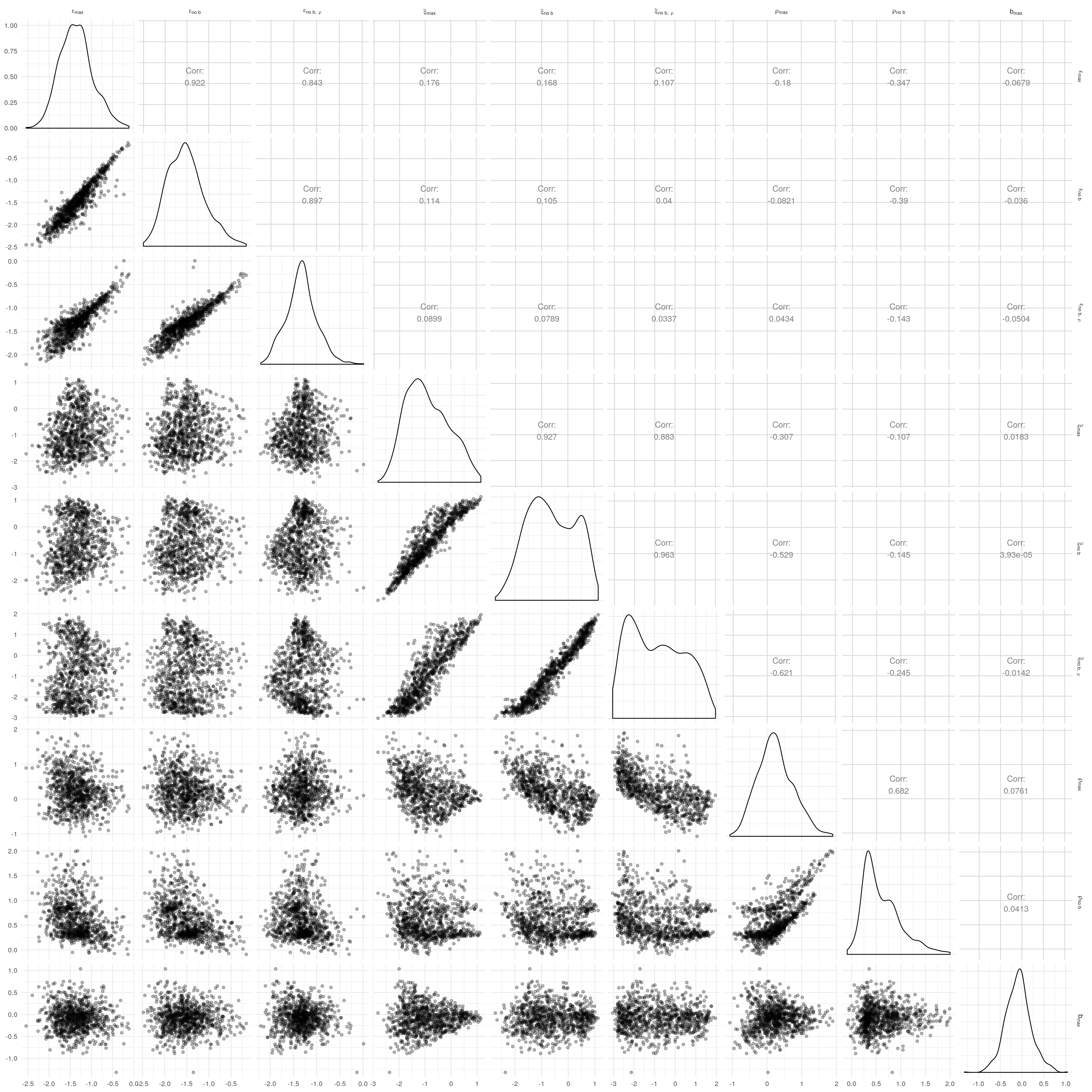
#> Call:psych::corr.p(r = psych::corr.test(filter(splt_rl_betas_sum,
#>     parameter == "rho_prm", block == 8)[, c("mean_par", "confidence")],
#>     method = "spearman")$r, n = 300, alpha = 0.005)
#> Correlation matrix
#>            mean_par confidence
#> mean_par       1.00       0.37
#> confidence     0.37       1.00
#> Sample Size
#> [1] 300
#> Probability values (Entries above the diagonal are adjusted for multiple tests.)
#>            mean_par confidence
#> mean_par          0          0
#> confidence        0          0
#>
#>  Confidence intervals based upon normal theory.  To get bootstrapped values, try cor.ci
#>             lower    r upper p
#> mn_pr-cnfdn  0.23 0.37   0.5 0
#> Call:psych::corr.p(r = psych::corr.test(filter(splt_rl_betas_sum,
#>     parameter == "xi_prm", block == 8)[, c("mean_par", "confidence")],
#>     method = "spearman")$r, n = 300, alpha = 0.005)
#> Correlation matrix
#>            mean_par confidence
#> mean_par       1.00      -0.34
#> confidence    -0.34       1.00
#> Sample Size
#> [1] 300
#> Probability values (Entries above the diagonal are adjusted for multiple tests.)
#>            mean_par confidence
#> mean_par          0          0
#> confidence        0          0
#>
#>  Confidence intervals based upon normal theory.  To get bootstrapped values, try cor.ci
#>             lower     r upper p
#> mn_pr-cnfdn -0.48 -0.34 -0.19 0
#> Call:psych::corr.p(r = psych::corr.test(filter(splt_rl_betas_sum,
#>     parameter == "ep_prm", block == 8)[, c("mean_par", "confidence")],
#>     method = "spearman")$r, n = 300, alpha = 0.005)
#> Correlation matrix
#>            mean_par confidence
#> mean_par       1.00      -0.12
#> confidence    -0.12       1.00
#> Sample Size
#> [1] 300
#> Probability values (Entries above the diagonal are adjusted for multiple tests.)
#>            mean_par confidence
#> mean_par       0.00       0.04
#> confidence     0.04       0.00
#>
#>  Confidence intervals based upon normal theory.  To get bootstrapped values, try cor.ci
#>             lower     r upper    p
#> mn_pr-cnfdn -0.28 -0.12  0.04 0.04
Relation of learning model to low-fi
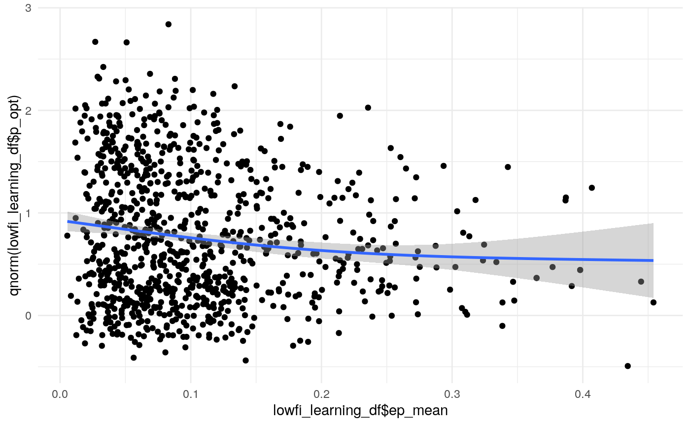
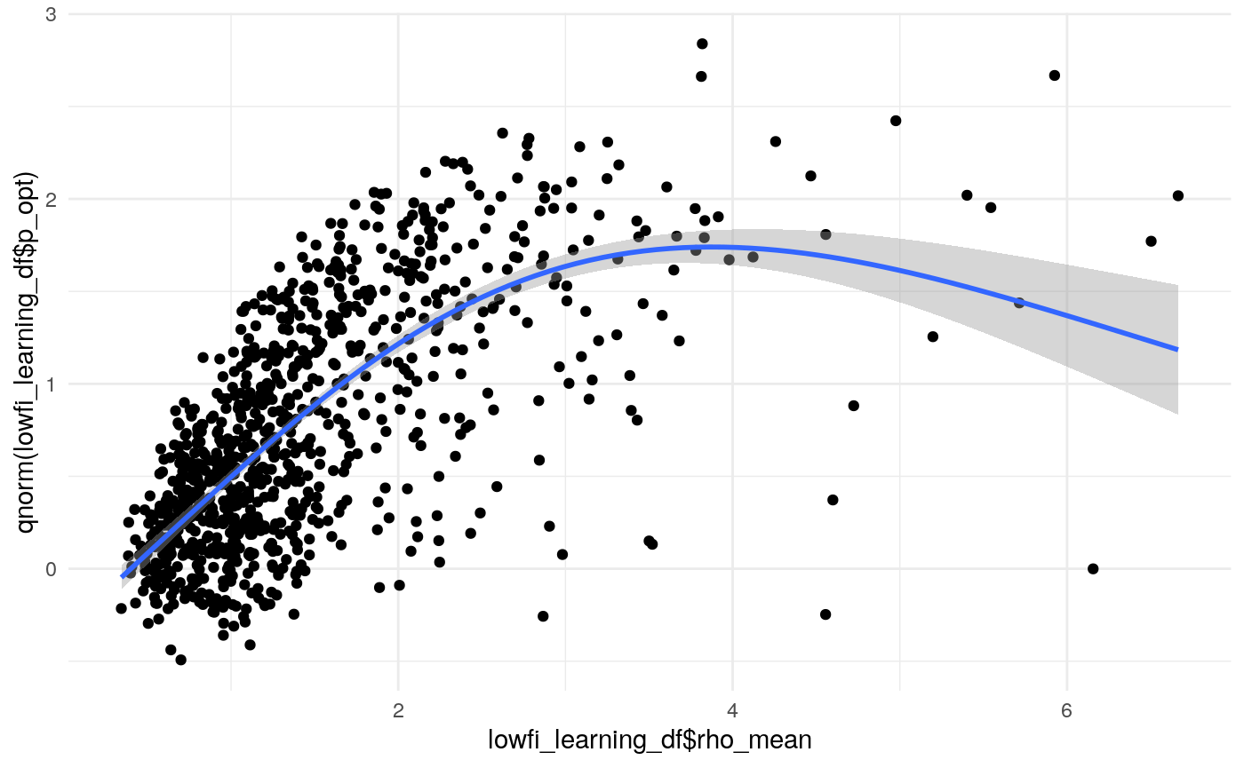
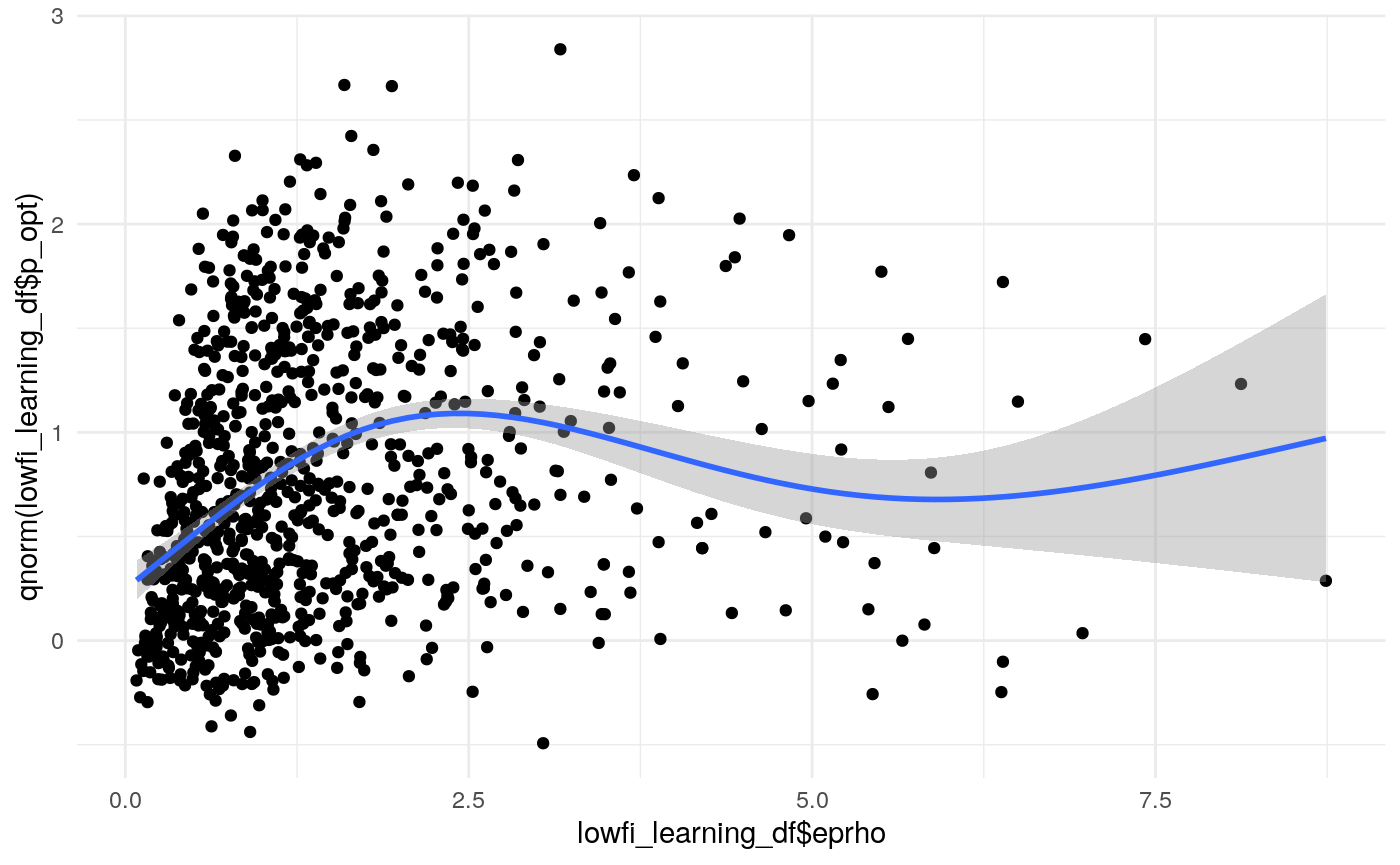
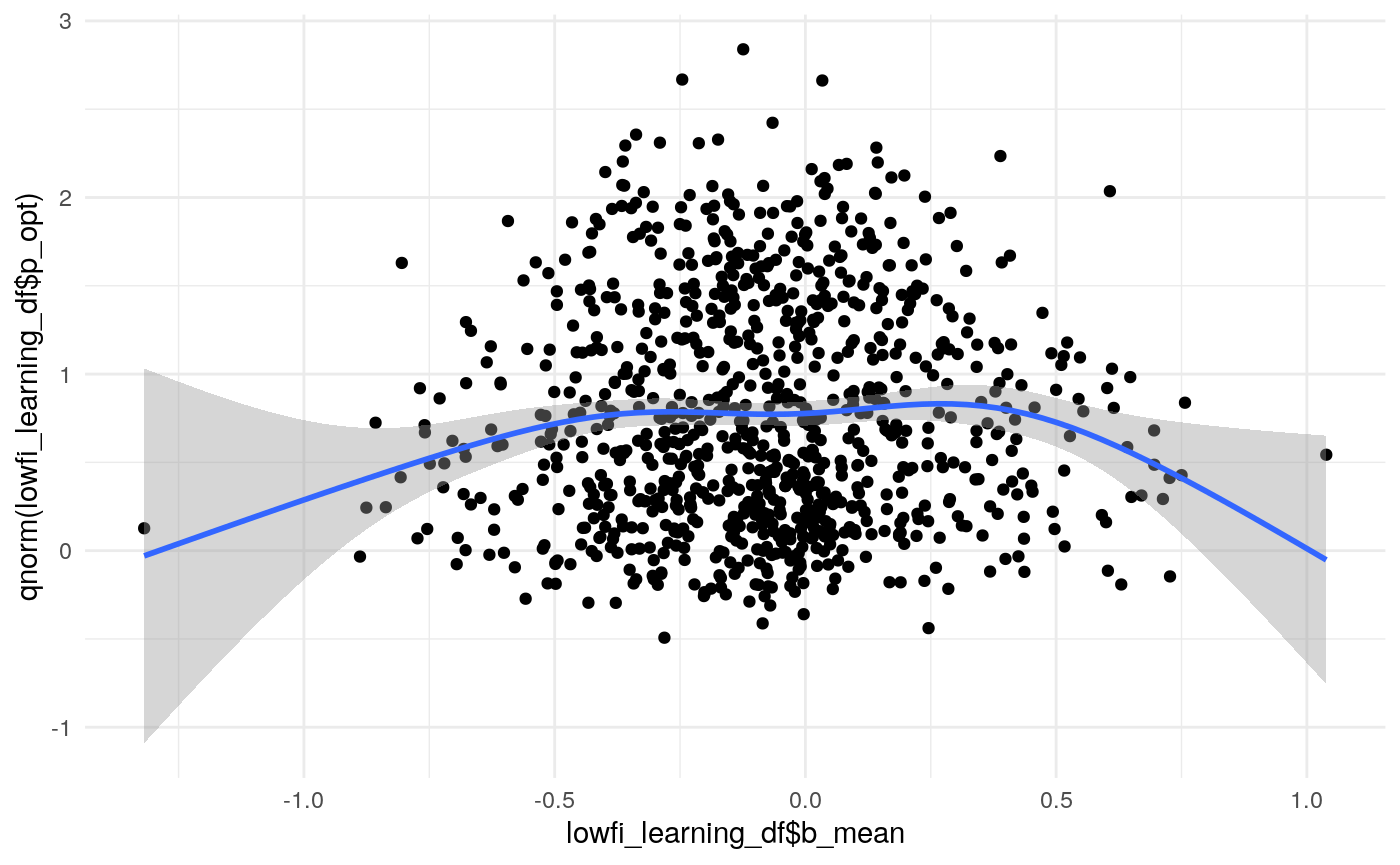
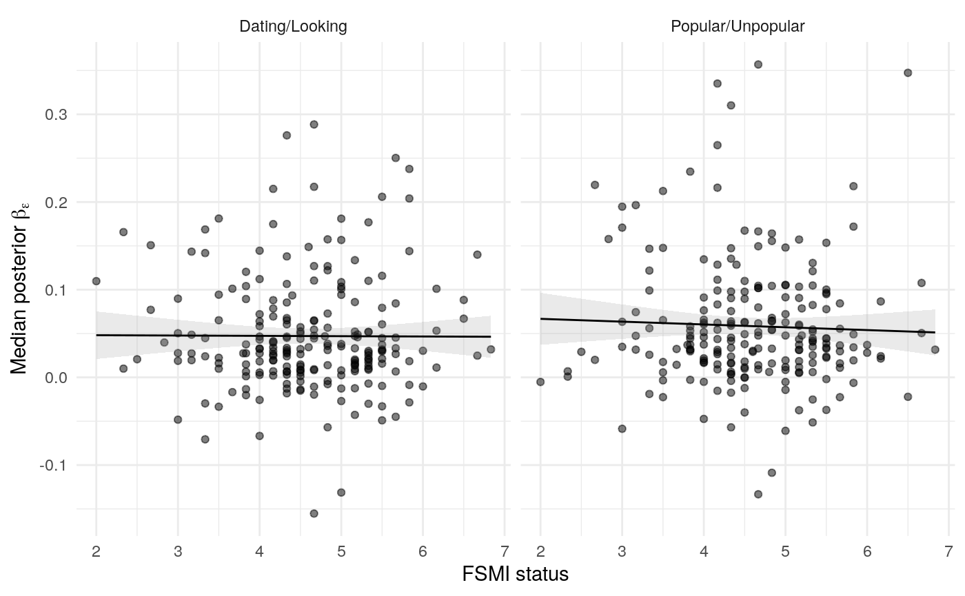
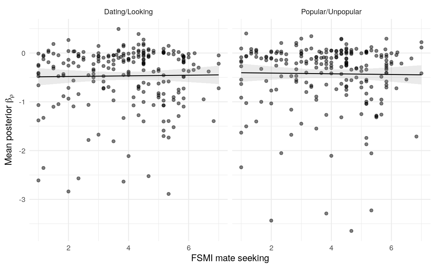
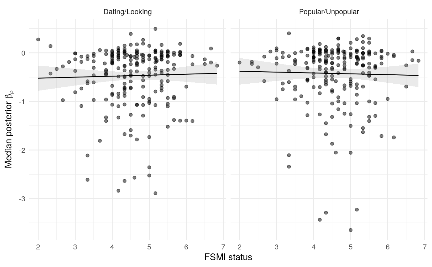
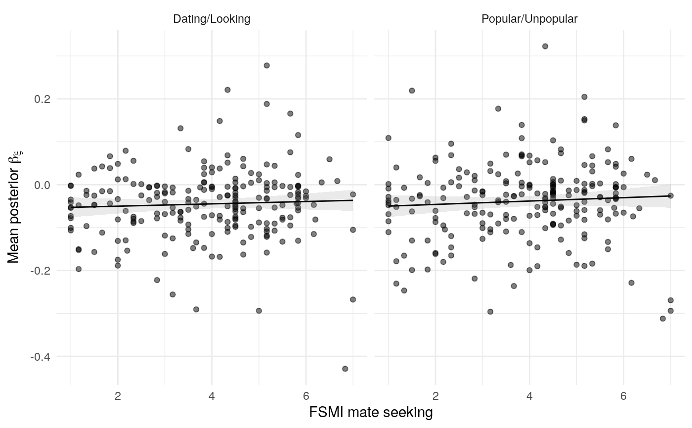
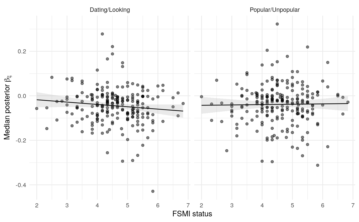
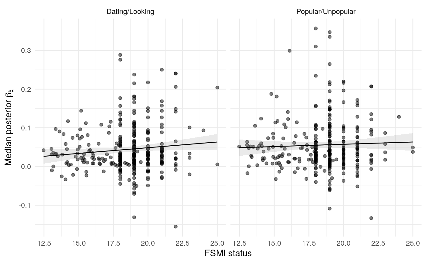
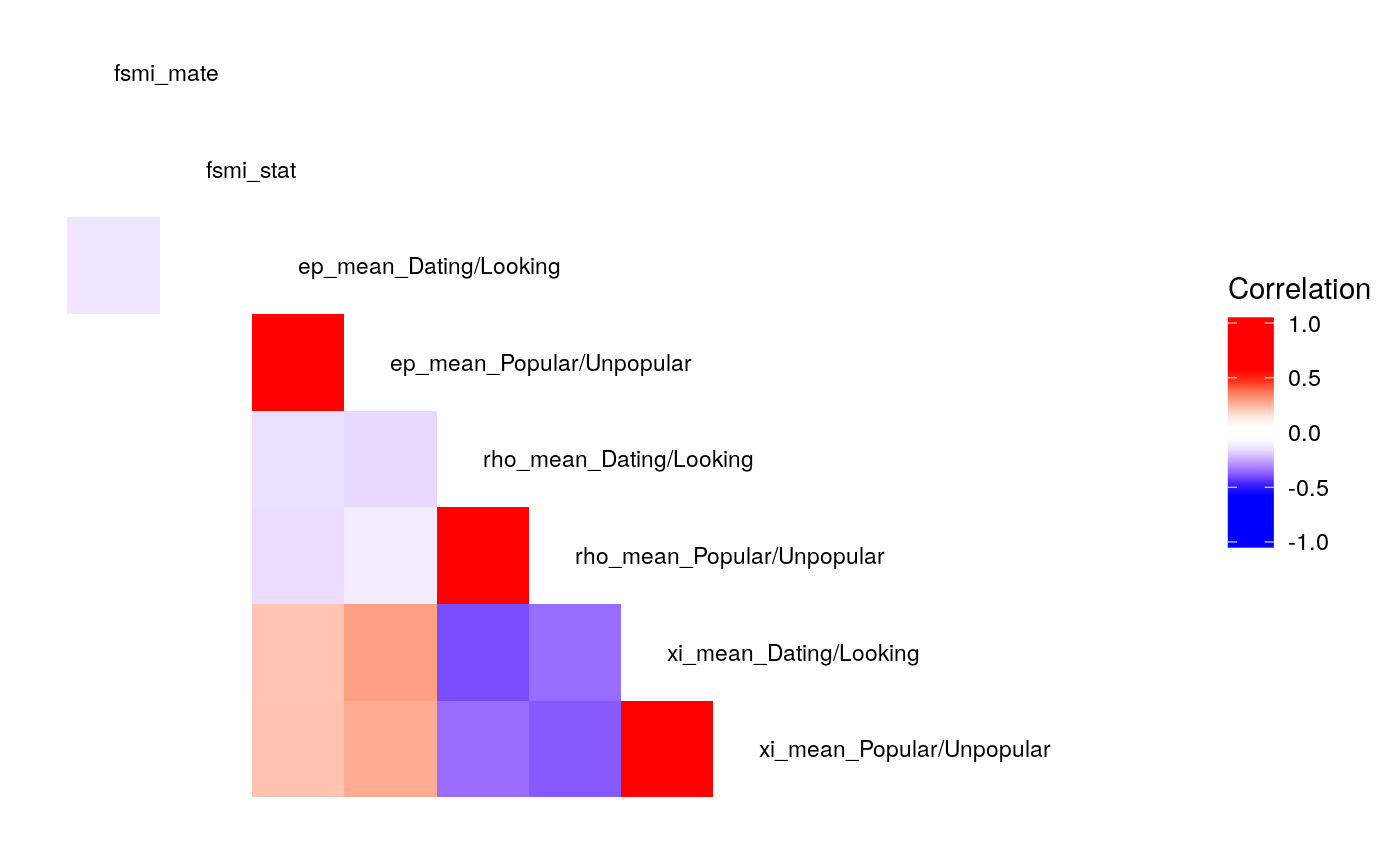
#> Call:psych::corr.test(x = select(ungroup(lowfi_learning_pdiffs_df_w),
#>     -id), method = "spearman")
#> Correlation matrix
#>                            fsmi_mate fsmi_stat ep_mean_Dating/Looking
#> fsmi_mate                       1.00      0.07                  -0.14
#> fsmi_stat                       0.07      1.00                  -0.06
#> ep_mean_Dating/Looking         -0.14     -0.06                   1.00
#> ep_mean_Popular/Unpopular      -0.08     -0.05                   0.73
#> rho_mean_Dating/Looking         0.02      0.01                  -0.15
#> rho_mean_Popular/Unpopular      0.02     -0.02                  -0.16
#> xi_mean_Dating/Looking          0.03     -0.05                   0.22
#> xi_mean_Popular/Unpopular       0.05     -0.02                   0.22
#>                            ep_mean_Popular/Unpopular rho_mean_Dating/Looking
#> fsmi_mate                                      -0.08                    0.02
#> fsmi_stat                                      -0.05                    0.01
#> ep_mean_Dating/Looking                          0.73                   -0.15
#> ep_mean_Popular/Unpopular                       1.00                   -0.17
#> rho_mean_Dating/Looking                        -0.17                    1.00
#> rho_mean_Popular/Unpopular                     -0.13                    0.92
#> xi_mean_Dating/Looking                          0.30                   -0.41
#> xi_mean_Popular/Unpopular                       0.27                   -0.35
#>                            rho_mean_Popular/Unpopular xi_mean_Dating/Looking
#> fsmi_mate                                        0.02                   0.03
#> fsmi_stat                                       -0.02                  -0.05
#> ep_mean_Dating/Looking                          -0.16                   0.22
#> ep_mean_Popular/Unpopular                       -0.13                   0.30
#> rho_mean_Dating/Looking                          0.92                  -0.41
#> rho_mean_Popular/Unpopular                       1.00                  -0.35
#> xi_mean_Dating/Looking                          -0.35                   1.00
#> xi_mean_Popular/Unpopular                       -0.39                   0.95
#>                            xi_mean_Popular/Unpopular
#> fsmi_mate                                       0.05
#> fsmi_stat                                      -0.02
#> ep_mean_Dating/Looking                          0.22
#> ep_mean_Popular/Unpopular                       0.27
#> rho_mean_Dating/Looking                        -0.35
#> rho_mean_Popular/Unpopular                     -0.39
#> xi_mean_Dating/Looking                          0.95
#> xi_mean_Popular/Unpopular                       1.00
#> Sample Size
#>                            fsmi_mate fsmi_stat ep_mean_Dating/Looking
#> fsmi_mate                        220       220                    220
#> fsmi_stat                        220       220                    220
#> ep_mean_Dating/Looking           220       220                    308
#> ep_mean_Popular/Unpopular        220       220                    308
#> rho_mean_Dating/Looking          220       220                    308
#> rho_mean_Popular/Unpopular       220       220                    308
#> xi_mean_Dating/Looking           220       220                    308
#> xi_mean_Popular/Unpopular        220       220                    308
#>                            ep_mean_Popular/Unpopular rho_mean_Dating/Looking
#> fsmi_mate                                        220                     220
#> fsmi_stat                                        220                     220
#> ep_mean_Dating/Looking                           308                     308
#> ep_mean_Popular/Unpopular                        308                     308
#> rho_mean_Dating/Looking                          308                     308
#> rho_mean_Popular/Unpopular                       308                     308
#> xi_mean_Dating/Looking                           308                     308
#> xi_mean_Popular/Unpopular                        308                     308
#>                            rho_mean_Popular/Unpopular xi_mean_Dating/Looking
#> fsmi_mate                                         220                    220
#> fsmi_stat                                         220                    220
#> ep_mean_Dating/Looking                            308                    308
#> ep_mean_Popular/Unpopular                         308                    308
#> rho_mean_Dating/Looking                           308                    308
#> rho_mean_Popular/Unpopular                        308                    308
#> xi_mean_Dating/Looking                            308                    308
#> xi_mean_Popular/Unpopular                         308                    308
#>                            xi_mean_Popular/Unpopular
#> fsmi_mate                                        220
#> fsmi_stat                                        220
#> ep_mean_Dating/Looking                           308
#> ep_mean_Popular/Unpopular                        308
#> rho_mean_Dating/Looking                          308
#> rho_mean_Popular/Unpopular                       308
#> xi_mean_Dating/Looking                           308
#> xi_mean_Popular/Unpopular                        308
#> Probability values (Entries above the diagonal are adjusted for multiple tests.)
#>                            fsmi_mate fsmi_stat ep_mean_Dating/Looking
#> fsmi_mate                       0.00      1.00                   0.46
#> fsmi_stat                       0.34      0.00                   1.00
#> ep_mean_Dating/Looking          0.04      0.37                   0.00
#> ep_mean_Popular/Unpopular       0.27      0.49                   0.00
#> rho_mean_Dating/Looking         0.74      0.88                   0.01
#> rho_mean_Popular/Unpopular      0.73      0.77                   0.01
#> xi_mean_Dating/Looking          0.67      0.47                   0.00
#> xi_mean_Popular/Unpopular       0.45      0.80                   0.00
#>                            ep_mean_Popular/Unpopular rho_mean_Dating/Looking
#> fsmi_mate                                       1.00                    1.00
#> fsmi_stat                                       1.00                    1.00
#> ep_mean_Dating/Looking                          0.00                    0.10
#> ep_mean_Popular/Unpopular                       0.00                    0.05
#> rho_mean_Dating/Looking                         0.00                    0.00
#> rho_mean_Popular/Unpopular                      0.02                    0.00
#> xi_mean_Dating/Looking                          0.00                    0.00
#> xi_mean_Popular/Unpopular                       0.00                    0.00
#>                            rho_mean_Popular/Unpopular xi_mean_Dating/Looking
#> fsmi_mate                                        1.00                      1
#> fsmi_stat                                        1.00                      1
#> ep_mean_Dating/Looking                           0.09                      0
#> ep_mean_Popular/Unpopular                        0.26                      0
#> rho_mean_Dating/Looking                          0.00                      0
#> rho_mean_Popular/Unpopular                       0.00                      0
#> xi_mean_Dating/Looking                           0.00                      0
#> xi_mean_Popular/Unpopular                        0.00                      0
#>                            xi_mean_Popular/Unpopular
#> fsmi_mate                                          1
#> fsmi_stat                                          1
#> ep_mean_Dating/Looking                             0
#> ep_mean_Popular/Unpopular                          0
#> rho_mean_Dating/Looking                            0
#> rho_mean_Popular/Unpopular                         0
#> xi_mean_Dating/Looking                             0
#> xi_mean_Popular/Unpopular                          0
#>
#>  To see confidence intervals of the correlations, print with the short=FALSE option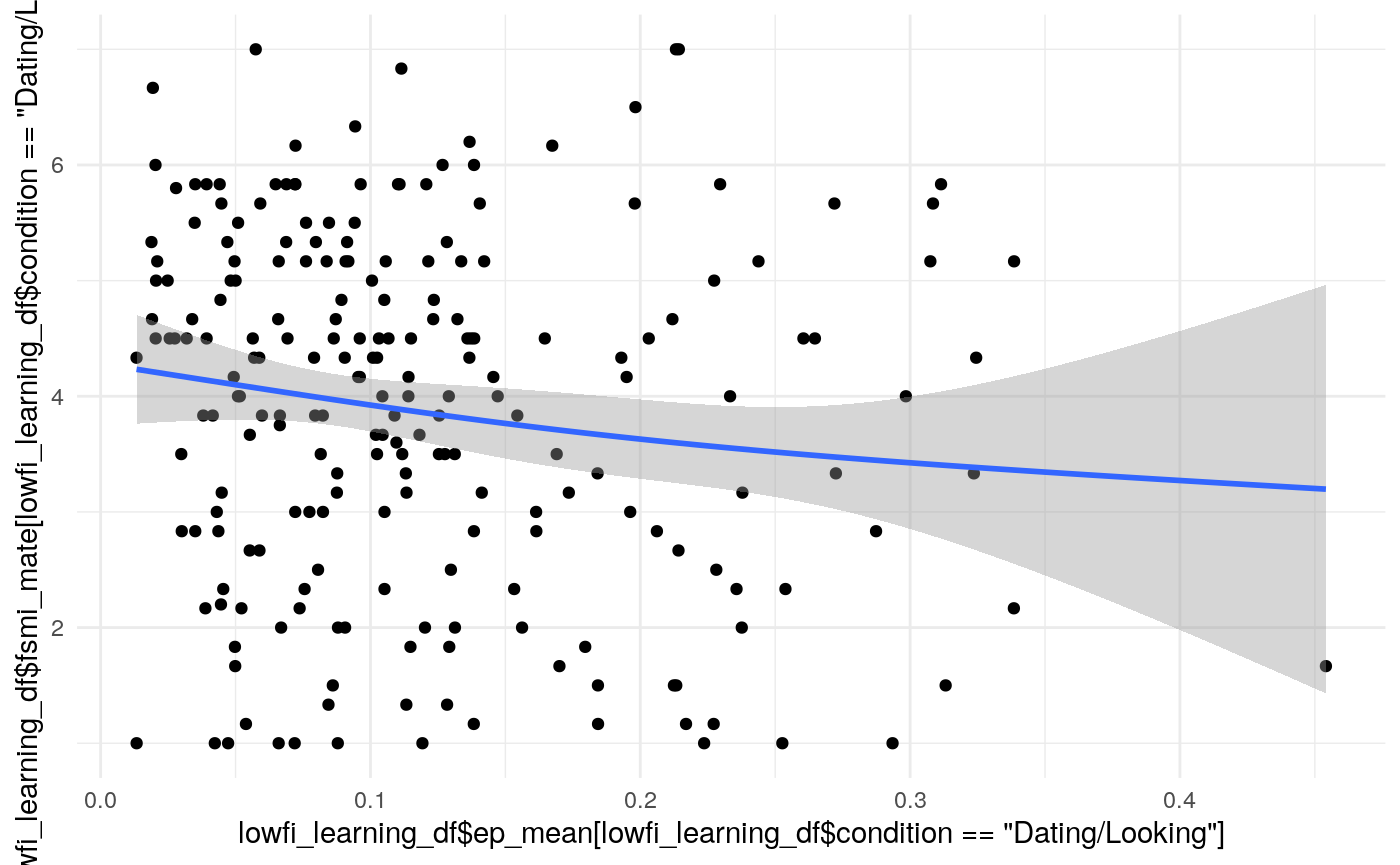
#>
#> Kendall's rank correlation tau
#>
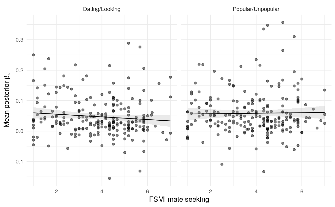
#> data: lowfi_learning_df$ep_mean[lowfi_learning_df$condition == "Dating/Looking"] and lowfi_learning_df$fsmi_mate[lowfi_learning_df$condition == "Dating/Looking"]
#> z = -2.2223, p-value = 0.02626
#> alternative hypothesis: true tau is not equal to 0
#> sample estimates:
#> tau
#> -0.1022479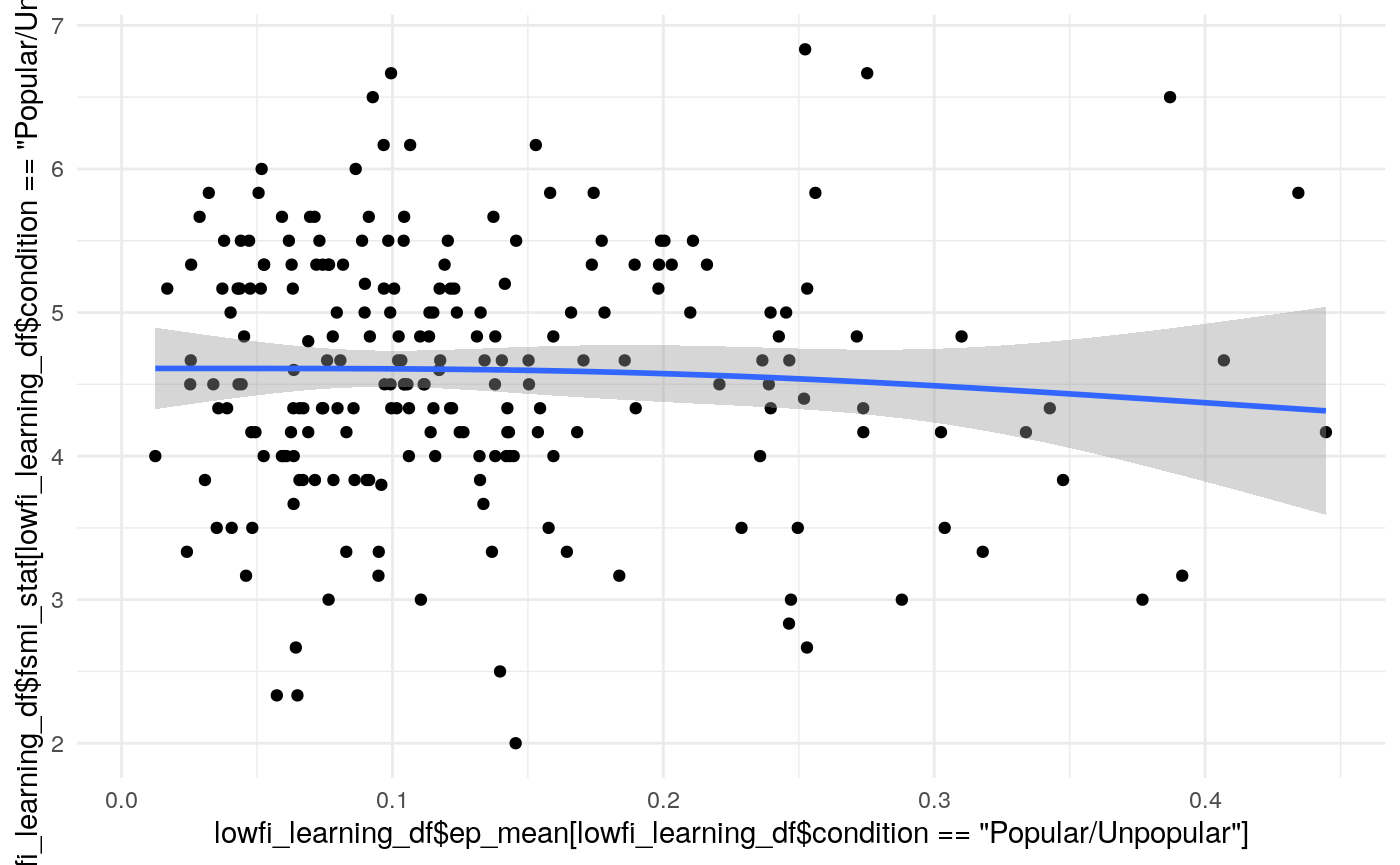
#>
#>  Kendall's rank correlation tau
#>
#> data:  lowfi_learning_df$ep_mean[lowfi_learning_df$condition == "Popular/Unpopular"] and lowfi_learning_df$fsmi_stat[lowfi_learning_df$condition == "Popular/Unpopular"]
#> z = -0.71608, p-value = 0.4739
#> alternative hypothesis: true tau is not equal to 0
#> sample estimates:
#>         tau
#> -0.03322081
Variance
#>   id:sample  stim_image      sample
#> 0.076362025 0.006069852 0.007163039
In a simple logistic regression, grouping responses by participant, nested in sample, and by stimulus image, it turns out that only 8% of the variance is due to differences in participants. Note, that this is for the average probability of choosing an optimal response. Another 1% and 1% of the variance is accounted for by sample and stimulus image, respectively.
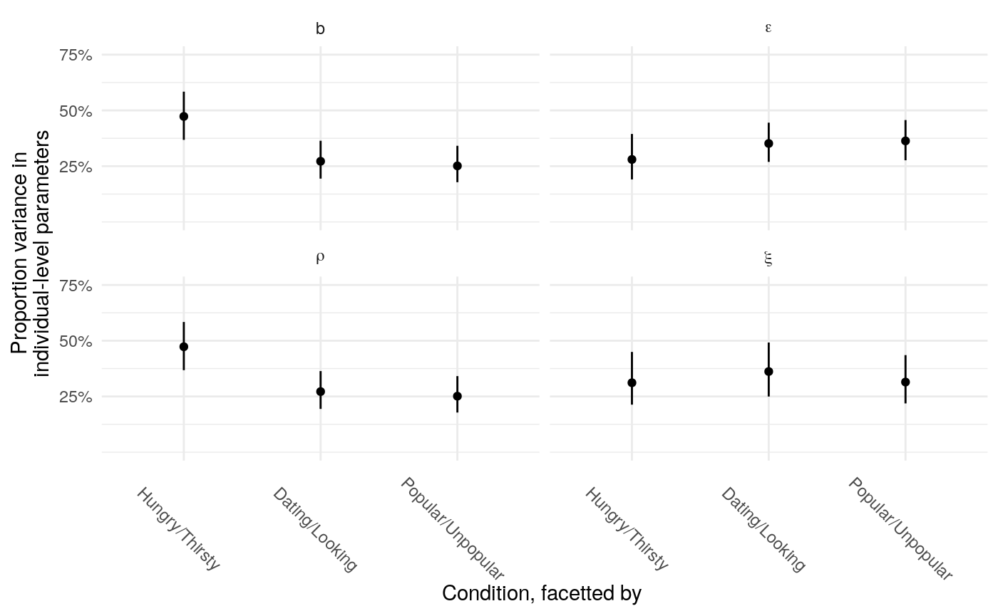
In the context of the learning model, it’s more difficult to estimate the proportion of total variance accounted for by individually-varying parameters, but there are a couple of ways to get a sense for how much variation in the individual parameters relative to the precision of those estimates. First, one can examine the proportion of variance accounted for by individual level parameters across each parameter and condition. This will tell you the relative proportion of variability across the three conditions.
One might also examine the variance of posterior means versus the total variance across iterations.
#>           [,1]      [,2]      [,3]
#> [1,] 0.3114072 0.1776992 0.1838759
#> [2,] 0.1776992 0.3850601 0.2467515
#> [3,] 0.1838759 0.2467515 0.3976845
#>          [,1]     [,2]     [,3]
#> [1,] 1.954619 1.811038 1.611297
#> [2,] 1.811038 2.250870 1.874122
#> [3,] 1.611297 1.874122 1.955437
#>           [,1]      [,2]      [,3]
#> [1,] 0.8937943 0.5617527 0.5396828
#> [2,] 0.5617527 0.5164993 0.4034440
#> [3,] 0.5396828 0.4034440 0.4765235
#>            [,1]       [,2]       [,3]
#> [1,] 0.12623682 0.04483997 0.05462949
#> [2,] 0.04483997 0.16033983 0.08227789
#> [3,] 0.05462949 0.08227789 0.18090651
#>           [,1]      [,2]      [,3]
#> [1,] 1.0000000 0.5131648 0.5225058
#> [2,] 0.5131648 1.0000000 0.6305598
#> [3,] 0.5225058 0.6305598 1.0000000
#>           [,1]      [,2]      [,3]
#> [1,] 1.0000000 0.8634185 0.8241809
#> [2,] 0.8634185 1.0000000 0.8933067
#> [3,] 0.8241809 0.8933067 1.0000000
#>           [,1]      [,2]      [,3]
#> [1,] 1.0000000 0.8267829 0.8269469
#> [2,] 0.8267829 1.0000000 0.8132166
#> [3,] 0.8269469 0.8132166 1.0000000
#>           [,1]      [,2]      [,3]
#> [1,] 1.0000000 0.3151748 0.3614989
#> [2,] 0.3151748 1.0000000 0.4830981
#> [3,] 0.3614989 0.4830981 1.0000000| var_means | var_tot | prop_var | |
|---|---|---|---|
| ep_1 | 0.12 | 0.32 | 0.37 |
| ep_2 | 0.17 | 0.39 | 0.45 |
| ep_3 | 0.18 | 0.40 | 0.45 |
| xi_1 | 0.98 | 2.08 | 0.47 |
| xi_2 | 1.21 | 2.45 | 0.49 |
| xi_3 | 1.04 | 2.10 | 0.49 |
| rho_1 | 0.43 | 0.92 | 0.47 |
| rho_2 | 0.25 | 0.53 | 0.47 |
| rho_3 | 0.23 | 0.49 | 0.47 |
| b_1 | 0.06 | 0.12 | 0.49 |
| b_2 | 0.09 | 0.16 | 0.56 |
| b_3 | 0.10 | 0.18 | 0.56 |
| par | ep_prm |
| X31 | 0.3362385 |
| X21 | 0.3127098 |
| par.1 | xi_prm |
| X31.1 | 0.2554012 |
| X21.1 | 0.2332147 |
| par.2 | rho_prm |
| X31.2 | 0.1670327 |
| X21.2 | 0.1533051 |
| par.3 | b |
| X31.3 | 0.4228785 |
| X21.3 | 0.4318277 |
So the proportion of variance due to the means of individual-level parameter posteriors tends to be highest for \(\xi\) and lowest for \(\rho\).
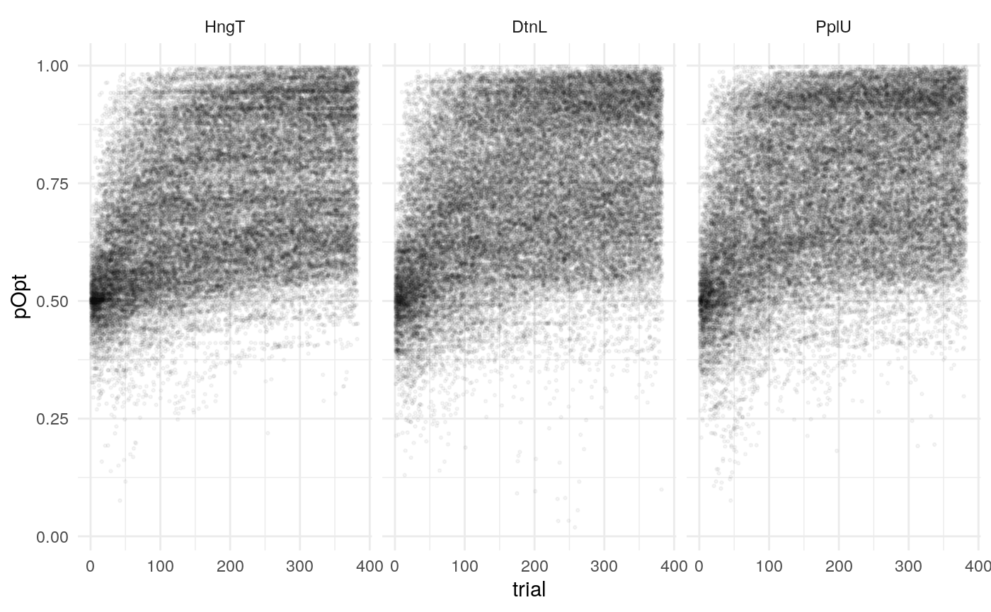
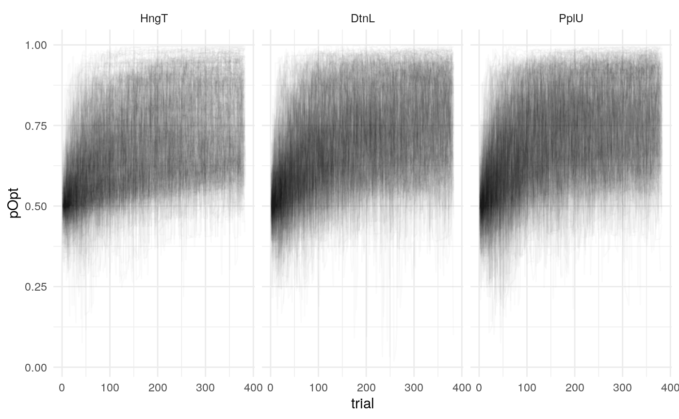
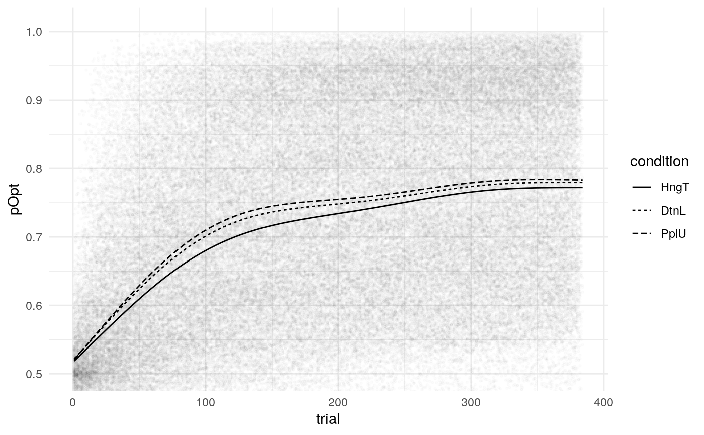
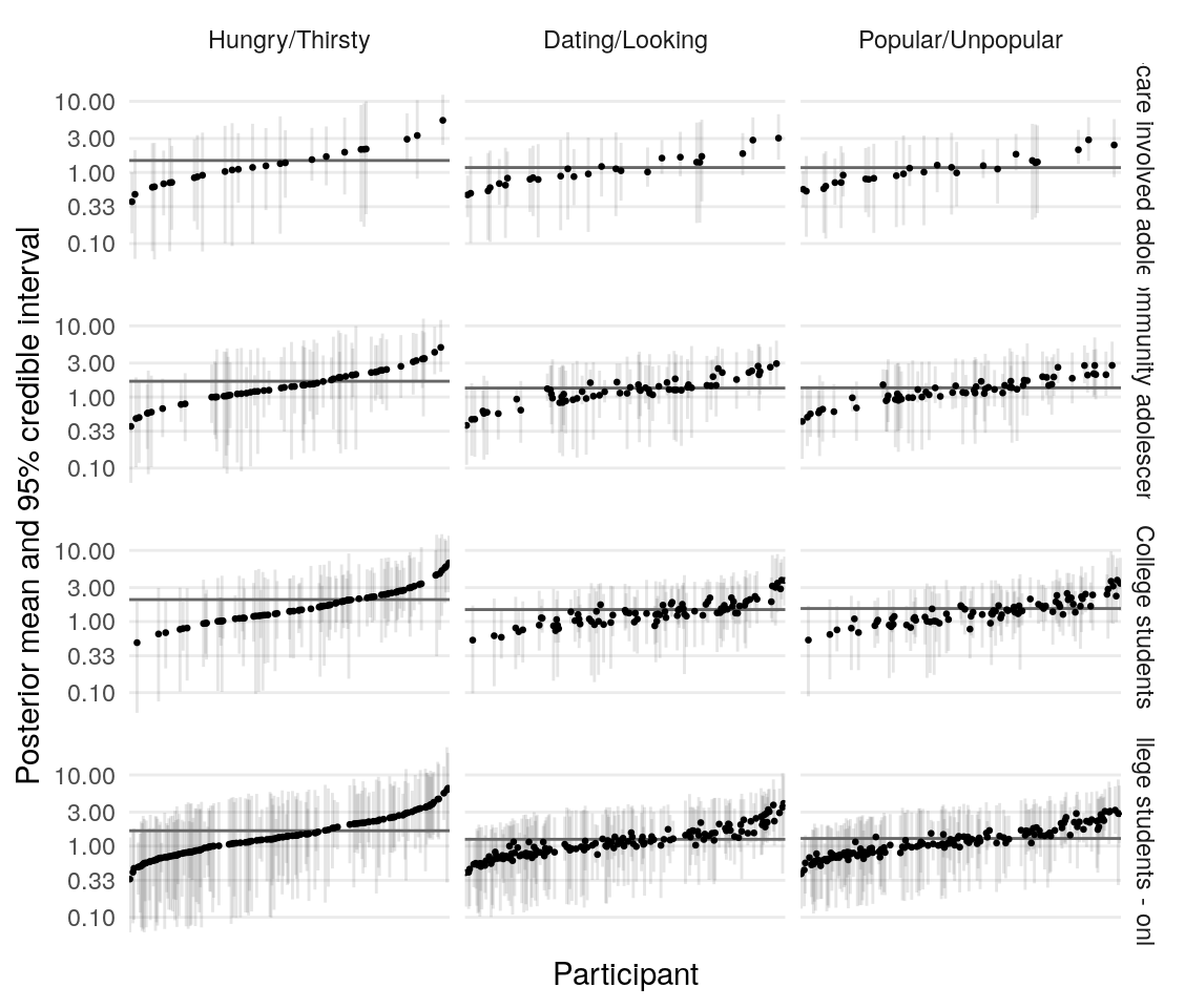
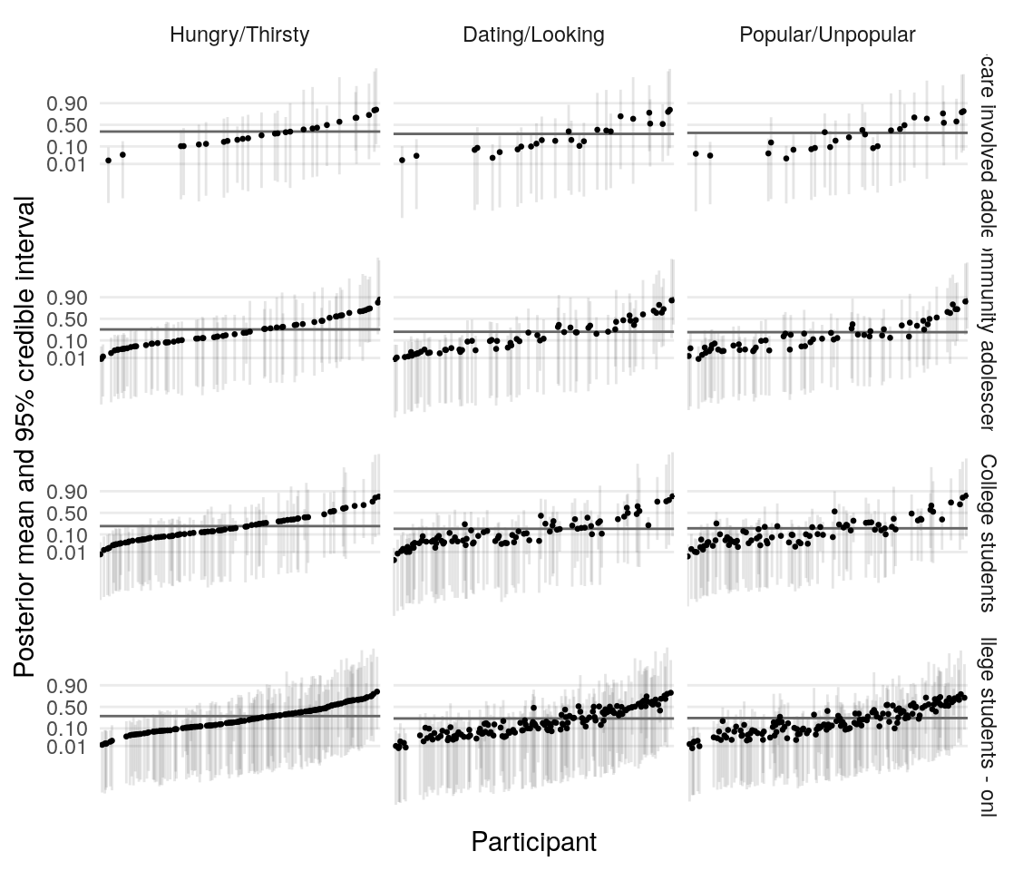
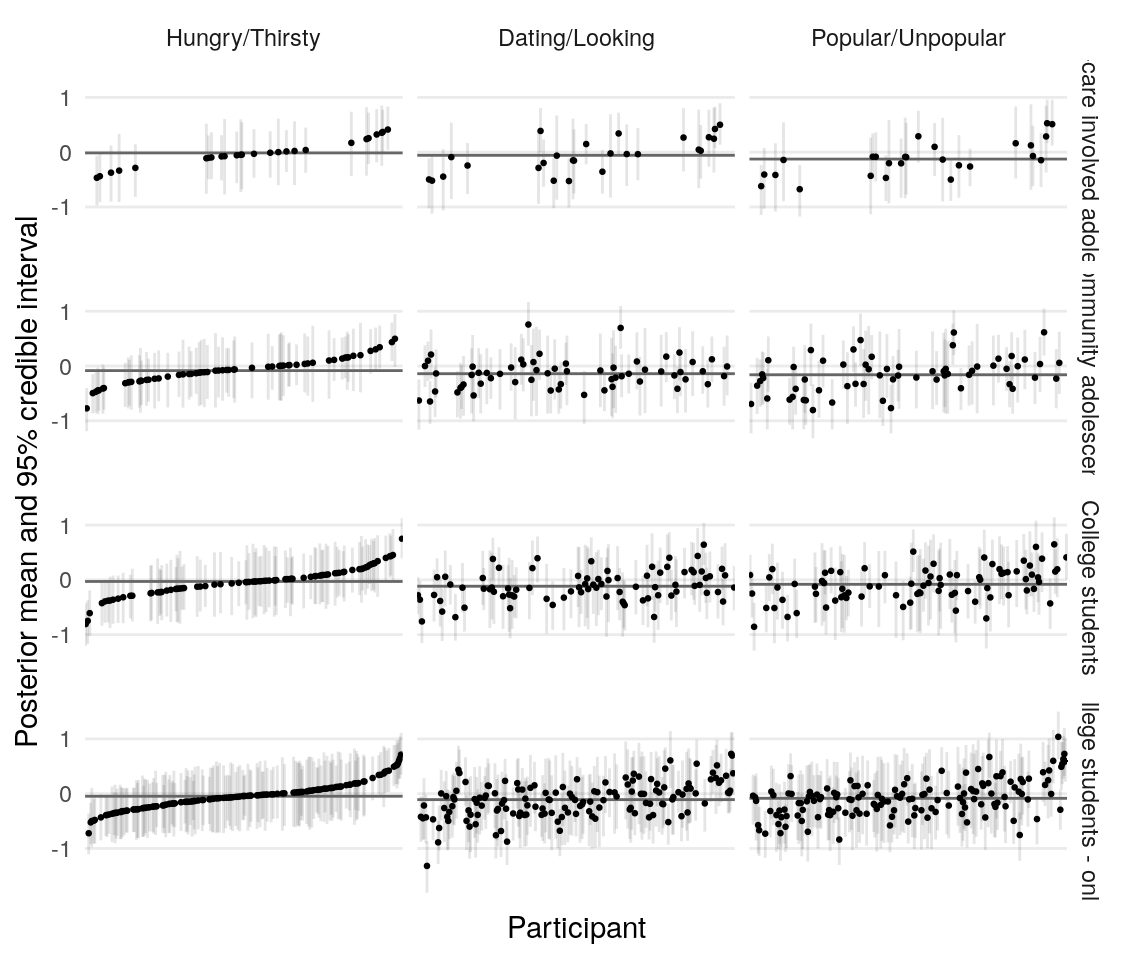
Model predicted behavior
Below is a plot of 313 model predicted runs, all using the exact same task structure (arbitrarily, the first run of the task). Behavior is guided by the mean parameter estimates, so any variabilility in behavior is due to the probabilistic nature of selecting either the right or left option based on the model’s current knowledge at some point during the task. Another way of framing this is that it is the behavior of the averge actor, in 313 identical, hypothetical runs.
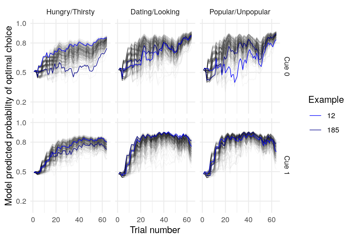
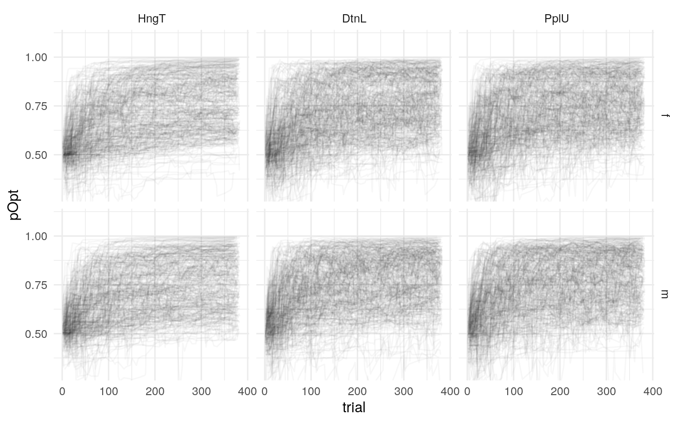
Individual probability trajectories

#> [[1]]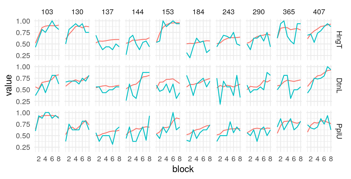
#>
#> [[2]]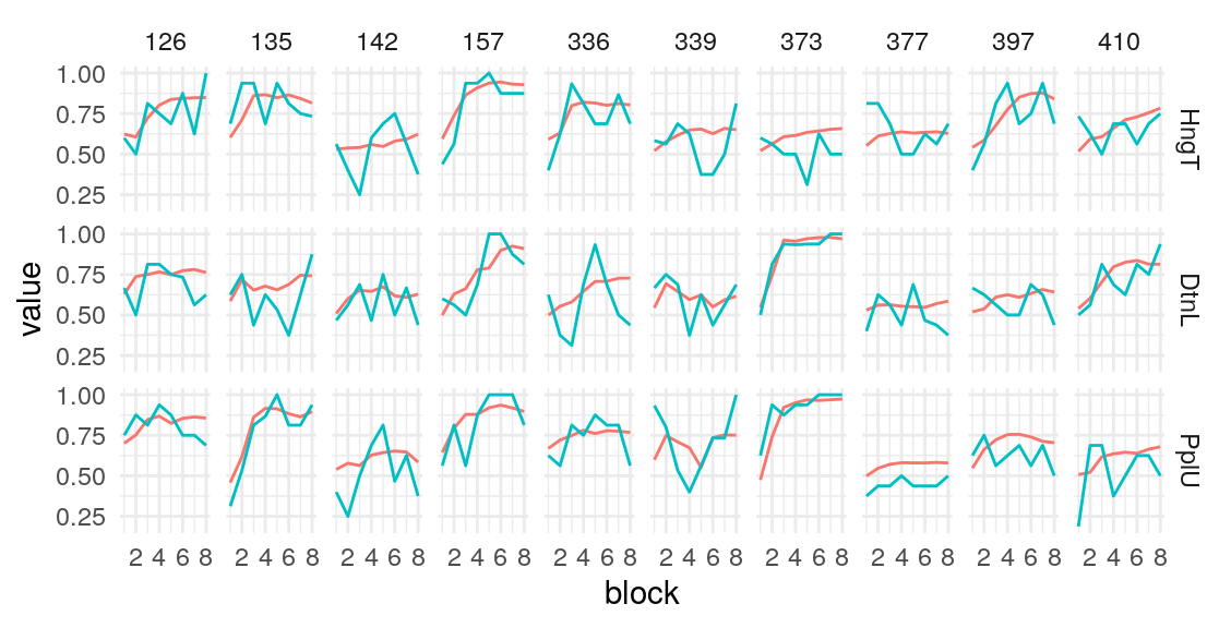
#>
#> [[3]]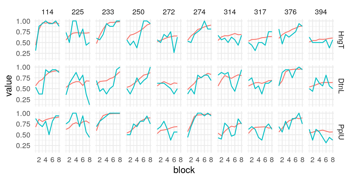
#>
#> [[4]]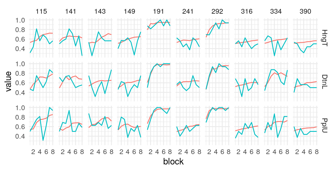
#>
#> [[5]]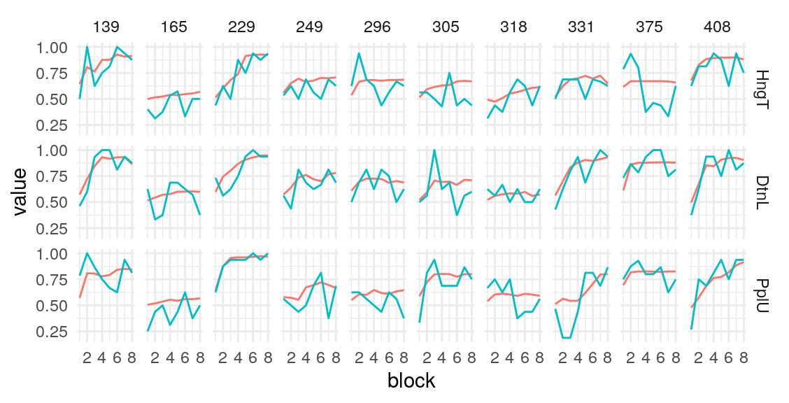
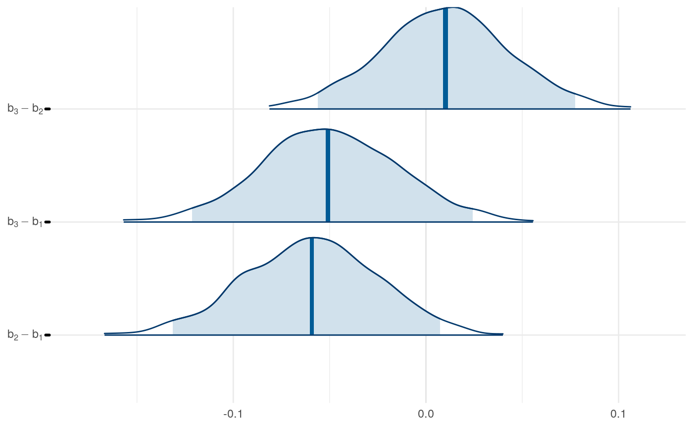
Given these model parameters, and the very strong assumption that nothing would purturb them from session to session, what would be the expected test-retest correlation for the differences between the H/T baseline and D/L or P/U conditions? The outcome of interest I’ll use is the average difference in the probability of choosing the optimal label in the last half of the run. This will over-estimate the true test-reliability because we’re using what is in practice an unknown latent parameter. Measurement error in any real situation will attenuate this true reliability. One way to assess this reliability is to draw random IDs (which in this case corresponds to simulated runs through the task), and then correlate the mean number of optimal presses in each condition across two sets of random draws. After all, since these simulations are all generating using the model parameters from the same participant, the rank-order of the mean probability of optimal press across the three conditions should be similar across simulations to the extent that the generated behavior is stable. A less ad hoc approach may be to use an interclass-correlation estimate to partition the variance into that systematically related to condition versus residual variance. In both cases, the estimate is middling, around .4 and .5 respectively. We can compare this to the observed reliability of the parameter estimates we obtain from the Bayesian models.
#>      2.5%       50%     97.5%
#> 0.2169802 0.2752571 0.3303462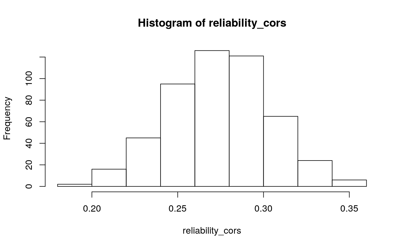
#> Linear mixed model fit by REML ['lmerMod']
#> Formula: mean_mean_p_opt ~ 1 + (1 | condition)
#>    Data: mean_modpred_ppressopt
#>
#> REML criterion at convergence: -3817.7
#>
#> Scaled residuals:
#>     Min      1Q  Median      3Q     Max
#> -4.8787 -0.5973  0.1317  0.6942  2.2393
#>
#> Random effects:
#>  Groups    Name        Variance  Std.Dev.
#>  condition (Intercept) 0.0005536 0.02353
#>  Residual              0.0009816 0.03133
#> Number of obs: 939, groups:  condition, 3
#>
#> Fixed effects:
#>             Estimate Std. Error t value
#> (Intercept)  0.78948    0.01362   57.95
#> [1] 0.3605915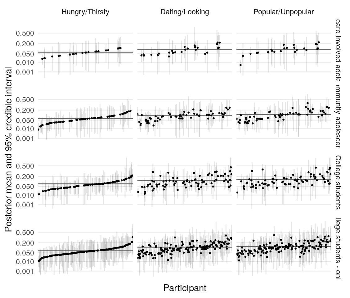
Acquiescence Bias Check
#> Call:psych::corr.test(x = cbind(splt_fsmi$fsmi_qs_67, splt_fsmi$dominance_prestige_18,
#>     splt_fsmi_ksrq_scored[, -5]), use = "pairwise.complete.obs",
#>     method = "spearman", adjust = "none")
#> Correlation matrix
#>                                 splt_fsmi$fsmi_qs_67
#> splt_fsmi$fsmi_qs_67                            1.00
#> splt_fsmi$dominance_prestige_18                -0.31
#> k_srq_admiration                               -0.23
#> k_srq_passivity                                 0.07
#> k_srq_sexual_relationships                     -0.16
#> k_srq_sociability                              -0.17
#>                                 splt_fsmi$dominance_prestige_18
#> splt_fsmi$fsmi_qs_67                                      -0.31
#> splt_fsmi$dominance_prestige_18                            1.00
#> k_srq_admiration                                           0.34
#> k_srq_passivity                                            0.00
#> k_srq_sexual_relationships                                 0.27
#> k_srq_sociability                                          0.35
#>                                 k_srq_admiration k_srq_passivity
#> splt_fsmi$fsmi_qs_67                       -0.23            0.07
#> splt_fsmi$dominance_prestige_18             0.34            0.00
#> k_srq_admiration                            1.00            0.01
#> k_srq_passivity                             0.01            1.00
#> k_srq_sexual_relationships                  0.49            0.06
#> k_srq_sociability                           0.45            0.11
#>                                 k_srq_sexual_relationships k_srq_sociability
#> splt_fsmi$fsmi_qs_67                                 -0.16             -0.17
#> splt_fsmi$dominance_prestige_18                       0.27              0.35
#> k_srq_admiration                                      0.49              0.45
#> k_srq_passivity                                       0.06              0.11
#> k_srq_sexual_relationships                            1.00              0.58
#> k_srq_sociability                                     0.58              1.00
#> Sample Size
#>                                 splt_fsmi$fsmi_qs_67
#> splt_fsmi$fsmi_qs_67                             140
#> splt_fsmi$dominance_prestige_18                  140
#> k_srq_admiration                                 138
#> k_srq_passivity                                  138
#> k_srq_sexual_relationships                       138
#> k_srq_sociability                                138
#>                                 splt_fsmi$dominance_prestige_18
#> splt_fsmi$fsmi_qs_67                                        140
#> splt_fsmi$dominance_prestige_18                             140
#> k_srq_admiration                                            138
#> k_srq_passivity                                             138
#> k_srq_sexual_relationships                                  138
#> k_srq_sociability                                           138
#>                                 k_srq_admiration k_srq_passivity
#> splt_fsmi$fsmi_qs_67                         138             138
#> splt_fsmi$dominance_prestige_18              138             138
#> k_srq_admiration                             320             320
#> k_srq_passivity                              320             320
#> k_srq_sexual_relationships                   320             320
#> k_srq_sociability                            320             320
#>                                 k_srq_sexual_relationships k_srq_sociability
#> splt_fsmi$fsmi_qs_67                                   138               138
#> splt_fsmi$dominance_prestige_18                        138               138
#> k_srq_admiration                                       320               320
#> k_srq_passivity                                        320               320
#> k_srq_sexual_relationships                             320               320
#> k_srq_sociability                                      320               320
#> Probability values (Entries above the diagonal are adjusted for multiple tests.)
#>                                 splt_fsmi$fsmi_qs_67
#> splt_fsmi$fsmi_qs_67                            0.00
#> splt_fsmi$dominance_prestige_18                 0.00
#> k_srq_admiration                                0.01
#> k_srq_passivity                                 0.43
#> k_srq_sexual_relationships                      0.06
#> k_srq_sociability                               0.05
#>                                 splt_fsmi$dominance_prestige_18
#> splt_fsmi$fsmi_qs_67                                       0.00
#> splt_fsmi$dominance_prestige_18                            0.00
#> k_srq_admiration                                           0.00
#> k_srq_passivity                                            0.97
#> k_srq_sexual_relationships                                 0.00
#> k_srq_sociability                                          0.00
#>                                 k_srq_admiration k_srq_passivity
#> splt_fsmi$fsmi_qs_67                        0.01            0.43
#> splt_fsmi$dominance_prestige_18             0.00            0.97
#> k_srq_admiration                            0.00            0.91
#> k_srq_passivity                             0.91            0.00
#> k_srq_sexual_relationships                  0.00            0.26
#> k_srq_sociability                           0.00            0.05
#>                                 k_srq_sexual_relationships k_srq_sociability
#> splt_fsmi$fsmi_qs_67                                  0.06              0.05
#> splt_fsmi$dominance_prestige_18                       0.00              0.00
#> k_srq_admiration                                      0.00              0.00
#> k_srq_passivity                                       0.26              0.05
#> k_srq_sexual_relationships                            0.00              0.00
#> k_srq_sociability                                     0.00              0.00
#>
#>  To see confidence intervals of the correlations, print with the short=FALSE option
Revelle, W. (2017). Psych: Procedures for Psychological, Psychometric, and Personality Research. Evanston, Illinois: Northwestern University. Retrieved from https://CRAN.R-project.org/package=psych
Zinbarg, R. E., Yovel, I., Revelle, W., & McDonald, R. P. (2006). Estimating Generalizability to a Latent Variable Common to All of a Scale’s Indicators: A Comparison of Estimators for ωh. Applied Psychological Measurement, 30(2), 121–144. doi:10.1177/0146621605278814