Fundamental Social Motives Confirmatory Factor Analysis
John Flournoy
2020-04-01
fsmi-cfa.RmdBelow, I begin to examine the fit of scales measuring behaviors, beliefs, attitudes, and strategies relevant to mate-seeking and status motives. After examining the item distributions to see if there are any very problematic subsets, I fit a confirmatory factor analysis to remaining scales. I also confirm that an exploratory factor analysis shows expected factor structure.
#>
#>          0        1-2        3-5        6-9 10 or more
#>        133         60         44         47         35
#>
#>         0       1-2       3-5 6 or more
#>       187        67        29        35
#>
#>  No Yes
#> 157  63
#>
#>          0        1-9      10-19      20-39 40 or more
#>        102         69         31         36         34
#>
#>         0         1         2 3 or more
#>       102        96        40        51
Checking Items
| Scale name | Sample | \(\alpha\) | \(\lambda\text{-6}\) | Mean | SD |
|---|---|---|---|---|---|
| (F) Mate-seeking | CSYA | 0.92 | 0.92 | 3.94 | 1.65 |
| CSYA-O | 0.85 | 0.85 | 3.86 | 1.46 | |
| (F) Status | CSYA | 0.67 | 0.68 | 4.71 | 0.85 |
| CSYA-O | 0.71 | 0.69 | 4.52 | 0.87 | |
| (D) Dominance | CSYA | 0.78 | 0.79 | 3.11 | 0.96 |
| CSYA-O | 0.84 | 0.84 | 3.62 | 1.03 | |
| (D) Presitige | CSYA | 0.83 | 0.86 | 5.21 | 0.82 |
| CSYA-O | 0.78 | 0.81 | 5.02 | 0.70 |
| keyname | sample | raw_alpha | G6(smc) | mean | sd |
|---|---|---|---|---|---|
| (K) Admiration | FCA | 0.89 | 0.88 | 5.59 | 1.38 |
| CA | 0.74 | 0.68 | 5.88 | 0.84 | |
| CSYA | 0.84 | 0.81 | 5.46 | 1.03 | |
| CSYA-O | 0.87 | 0.84 | 5.40 | 1.04 | |
| (K) Passivity | FCA | 0.72 | 0.66 | 3.07 | 1.22 |
| CA | 0.81 | 0.74 | 2.92 | 1.38 | |
| CSYA | 0.75 | 0.70 | 3.27 | 1.27 | |
| CSYA-O | 0.80 | 0.73 | 3.20 | 1.27 | |
| (K) Sexual Rel. | FCA | 0.76 | 0.76 | 5.22 | 1.27 |
| CA | 0.80 | 0.74 | 5.25 | 1.33 | |
| CSYA | 0.77 | 0.72 | 5.62 | 1.10 | |
| CSYA-O | 0.73 | 0.66 | 5.52 | 1.17 | |
| (K) Sociability | FCA | 0.57 | 0.49 | 4.96 | 1.18 |
| CA | 0.51 | 0.47 | 5.06 | 1.16 | |
| CSYA | 0.51 | 0.42 | 5.51 | 1.01 | |
| CSYA-O | 0.69 | 0.62 | 5.24 | 1.22 |
| keyname | sample | raw_alpha | G6(smc) | mean | sd |
|---|---|---|---|---|---|
| (U) -Urgency | FCA | 0.87 | 0.90 | 2.86 | 0.61 |
| CA | 0.89 | 0.91 | 2.91 | 0.63 | |
| CSYA | 0.87 | 0.89 | 2.76 | 0.56 | |
| CSYA-O | 0.88 | 0.89 | 2.60 | 0.56 | |
| (U) Premeditation | FCA | 0.78 | 0.86 | 3.04 | 0.45 |
| CA | 0.83 | 0.87 | 3.04 | 0.49 | |
| CSYA | 0.71 | 0.81 | 3.15 | 0.37 | |
| CSYA-O | 0.82 | 0.85 | 3.09 | 0.43 | |
| (U) Perseverance | FCA | 0.84 | 0.88 | 2.79 | 0.55 |
| CA | 0.80 | 0.84 | 3.00 | 0.47 | |
| CSYA | 0.84 | 0.89 | 3.14 | 0.48 | |
| CSYA-O | 0.79 | 0.81 | 3.04 | 0.42 | |
| (U) Sensation S. | FCA | 0.77 | 0.86 | 2.27 | 0.50 |
| CA | 0.80 | 0.87 | 2.24 | 0.57 | |
| CSYA | 0.80 | 0.87 | 2.07 | 0.49 | |
| CSYA-O | 0.83 | 0.86 | 2.25 | 0.56 | |
| (U) +Urgency | FCA | 0.86 | 0.94 | 3.17 | 0.46 |
| CA | 0.88 | 0.92 | 3.16 | 0.51 | |
| CSYA | 0.84 | 0.90 | 3.06 | 0.43 | |
| CSYA-O | 0.87 | 0.90 | 2.93 | 0.51 |
FSMI
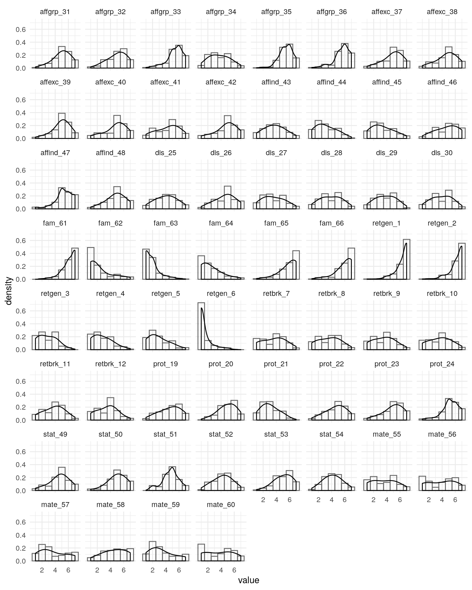
The CFA will not include kin care (missing data), family care (highly skewed), and mate retention general (highly skewed).
Confirmatory factor analyses and exploration
FSMI
| Df | AIC | BIC | Chisq | Chisq diff | Df diff | Pr(>Chisq) | cfi | rmsea | mfi | |
|---|---|---|---|---|---|---|---|---|---|---|
| fsmi_cfa_method | 1004 | 35242.29 | 35992.85 | 1678.665 | NA | NA | NA | 0.864 | 0.055 | 0.222 |
| fsmi_cfa | 1052 | 35492.99 | 36079.80 | 2025.366 | 260.673 | 48 | 0 | 0.804 | 0.064 | 0.114 |
#> lavaan 0.6-5 ended normally after 88 iterations
#>
#> Estimator ML
#> Optimization method NLMINB
#> Number of free parameters 172
#>
#> Used Total
#> Number of observations 224 334
#> Number of missing patterns 22
#>
#> Model Test User Model:
#> Standard Robust
#> Test Statistic 2025.366 1911.181
#> Degrees of freedom 1052 1052
#> P-value (Chi-square) 0.000 0.000
#> Scaling correction factor 1.060
#> for the Yuan-Bentler correction (Mplus variant)
#>
#> Parameter Estimates:
#>
#> Information Observed
#> Observed information based on Hessian
#> Standard errors Robust.huber.white
#>
#> Latent Variables:
#> Estimate Std.Err z-value P(>|z|) Std.lv Std.all
#> fsmi_affgrp =~
#> fsmi_qs_31 0.926 0.096 9.687 0.000 0.926 0.692
#> fsmi_qs_32 1.097 0.088 12.487 0.000 1.097 0.769
#> fsmi_qs_33 1.048 0.090 11.653 0.000 1.048 0.827
#> fsmi_qs_34 -0.702 0.133 -5.286 0.000 -0.702 -0.464
#> fsmi_qs_35 0.503 0.093 5.416 0.000 0.503 0.472
#> fsmi_qs_36 0.603 0.117 5.161 0.000 0.603 0.486
#> fsmi_affexc =~
#> fsmi_qs_37 1.160 0.098 11.861 0.000 1.160 0.790
#> fsmi_qs_38 1.225 0.091 13.453 0.000 1.225 0.807
#> fsmi_qs_39 1.007 0.101 9.981 0.000 1.007 0.766
#> fsmi_qs_40 1.029 0.133 7.726 0.000 1.029 0.641
#> fsmi_qs_41 0.994 0.126 7.893 0.000 0.994 0.590
#> fsmi_qs_42 0.957 0.151 6.359 0.000 0.957 0.612
#> fsmi_affind =~
#> fsmi_qs_43 1.190 0.117 10.130 0.000 1.190 0.751
#> fsmi_qs_44 0.971 0.118 8.237 0.000 0.971 0.645
#> fsmi_qs_45 0.906 0.121 7.458 0.000 0.906 0.557
#> fsmi_qs_46 1.180 0.116 10.128 0.000 1.180 0.708
#> fsmi_qs_47 0.879 0.126 6.949 0.000 0.879 0.635
#> fsmi_qs_48 1.112 0.115 9.641 0.000 1.112 0.759
#> fsmi_dis =~
#> fsmi_qs_25 0.895 0.127 7.077 0.000 0.895 0.563
#> fsmi_qs_26 0.947 0.117 8.071 0.000 0.947 0.616
#> fsmi_qs_27 0.981 0.136 7.232 0.000 0.981 0.602
#> fsmi_qs_28 -1.222 0.093 -13.115 0.000 -1.222 -0.764
#> fsmi_qs_29 -1.031 0.105 -9.835 0.000 -1.031 -0.683
#> fsmi_qs_30 -1.224 0.096 -12.775 0.000 -1.224 -0.785
#> fsmi_retbrk =~
#> fsmi_qs_7 1.450 0.072 20.035 0.000 1.450 0.840
#> fsmi_qs_8 1.133 0.109 10.351 0.000 1.133 0.684
#> fsmi_qs_9 1.391 0.085 16.403 0.000 1.391 0.854
#> fsmi_qs_10 1.459 0.084 17.289 0.000 1.459 0.854
#> fsmi_qs_11 0.890 0.108 8.248 0.000 0.890 0.575
#> fsmi_qs_12 1.125 0.099 11.398 0.000 1.125 0.730
#> fsmi_prot =~
#> fsmi_qs_19 1.276 0.085 14.931 0.000 1.276 0.805
#> fsmi_qs_20 0.944 0.086 10.928 0.000 0.944 0.711
#> fsmi_qs_21 -0.671 0.105 -6.416 0.000 -0.671 -0.503
#> fsmi_qs_22 1.131 0.089 12.770 0.000 1.131 0.750
#> fsmi_qs_23 1.207 0.091 13.257 0.000 1.207 0.797
#> fsmi_qs_24 0.977 0.086 11.365 0.000 0.977 0.735
#> fsmi_stat =~
#> fsmi_qs_49 0.824 0.130 6.342 0.000 0.824 0.569
#> fsmi_qs_50 0.724 0.119 6.090 0.000 0.724 0.528
#> fsmi_qs_51 0.761 0.099 7.697 0.000 0.761 0.607
#> fsmi_qs_52 0.810 0.122 6.667 0.000 0.810 0.574
#> fsmi_qs_53 0.801 0.109 7.336 0.000 0.801 0.594
#> fsmi_qs_54 -0.408 0.155 -2.628 0.009 -0.408 -0.296
#> fsmi_mate =~
#> fsmi_qs_55 1.403 0.092 15.285 0.000 1.403 0.761
#> fsmi_qs_56 1.895 0.076 25.053 0.000 1.895 0.914
#> fsmi_qs_57 -1.427 0.112 -12.732 0.000 -1.427 -0.720
#> fsmi_qs_58 -1.013 0.121 -8.372 0.000 -1.013 -0.572
#> fsmi_qs_59 -0.913 0.133 -6.865 0.000 -0.913 -0.501
#> fsmi_qs_60 1.901 0.068 28.073 0.000 1.901 0.916
#>
#> Covariances:
#> Estimate Std.Err z-value P(>|z|) Std.lv Std.all
#> fsmi_affgrp ~~
#> fsmi_affexc 0.431 0.091 4.714 0.000 0.431 0.431
#> fsmi_affind -0.402 0.096 -4.163 0.000 -0.402 -0.402
#> fsmi_dis -0.131 0.073 -1.789 0.074 -0.131 -0.131
#> fsmi_retbrk 0.150 0.081 1.847 0.065 0.150 0.150
#> fsmi_prot 0.190 0.086 2.222 0.026 0.190 0.190
#> fsmi_stat 0.415 0.102 4.090 0.000 0.415 0.415
#> fsmi_mate 0.199 0.071 2.785 0.005 0.199 0.199
#> fsmi_affexc ~~
#> fsmi_affind -0.166 0.091 -1.825 0.068 -0.166 -0.166
#> fsmi_dis 0.062 0.086 0.721 0.471 0.062 0.062
#> fsmi_retbrk 0.278 0.094 2.955 0.003 0.278 0.278
#> fsmi_prot 0.151 0.087 1.741 0.082 0.151 0.151
#> fsmi_stat 0.334 0.114 2.919 0.004 0.334 0.334
#> fsmi_mate 0.201 0.077 2.618 0.009 0.201 0.201
#> fsmi_affind ~~
#> fsmi_dis 0.089 0.087 1.020 0.308 0.089 0.089
#> fsmi_retbrk 0.103 0.084 1.226 0.220 0.103 0.103
#> fsmi_prot 0.141 0.094 1.501 0.133 0.141 0.141
#> fsmi_stat -0.011 0.106 -0.103 0.918 -0.011 -0.011
#> fsmi_mate -0.091 0.074 -1.217 0.224 -0.091 -0.091
#> fsmi_dis ~~
#> fsmi_retbrk -0.053 0.094 -0.566 0.571 -0.053 -0.053
#> fsmi_prot 0.220 0.096 2.276 0.023 0.220 0.220
#> fsmi_stat -0.025 0.096 -0.255 0.799 -0.025 -0.025
#> fsmi_mate -0.090 0.080 -1.129 0.259 -0.090 -0.090
#> fsmi_retbrk ~~
#> fsmi_prot 0.096 0.087 1.104 0.270 0.096 0.096
#> fsmi_stat 0.083 0.091 0.908 0.364 0.083 0.083
#> fsmi_mate 0.378 0.072 5.238 0.000 0.378 0.378
#> fsmi_prot ~~
#> fsmi_stat 0.331 0.085 3.893 0.000 0.331 0.331
#> fsmi_mate -0.119 0.079 -1.504 0.132 -0.119 -0.119
#> fsmi_stat ~~
#> fsmi_mate 0.093 0.087 1.066 0.287 0.093 0.093
#>
#> Intercepts:
#> Estimate Std.Err z-value P(>|z|) Std.lv Std.all
#> .fsmi_qs_31 5.034 0.090 56.161 0.000 5.034 3.760
#> .fsmi_qs_32 5.000 0.095 52.449 0.000 5.000 3.504
#> .fsmi_qs_33 5.437 0.085 64.272 0.000 5.437 4.294
#> .fsmi_qs_34 3.741 0.101 36.999 0.000 3.741 2.472
#> .fsmi_qs_35 5.478 0.071 77.005 0.000 5.478 5.145
#> .fsmi_qs_36 5.594 0.083 67.554 0.000 5.594 4.514
#> .fsmi_qs_37 4.904 0.099 49.670 0.000 4.904 3.342
#> .fsmi_qs_38 4.713 0.102 46.083 0.000 4.713 3.104
#> .fsmi_qs_39 4.945 0.088 55.939 0.000 4.945 3.764
#> .fsmi_qs_40 4.801 0.108 44.365 0.000 4.801 2.988
#> .fsmi_qs_41 4.339 0.114 38.133 0.000 4.339 2.574
#> .fsmi_qs_42 4.832 0.105 45.857 0.000 4.832 3.087
#> .fsmi_qs_43 3.717 0.106 35.054 0.000 3.717 2.347
#> .fsmi_qs_44 3.112 0.101 30.806 0.000 3.112 2.066
#> .fsmi_qs_45 3.319 0.109 30.488 0.000 3.319 2.041
#> .fsmi_qs_46 4.741 0.112 42.466 0.000 4.741 2.844
#> .fsmi_qs_47 5.332 0.093 57.608 0.000 5.332 3.854
#> .fsmi_qs_48 4.795 0.098 48.993 0.000 4.795 3.273
#> .fsmi_qs_25 4.045 0.106 38.030 0.000 4.045 2.541
#> .fsmi_qs_26 4.607 0.103 44.725 0.000 4.607 2.999
#> .fsmi_qs_27 3.562 0.109 32.653 0.000 3.562 2.185
#> .fsmi_qs_28 3.884 0.107 36.198 0.000 3.884 2.429
#> .fsmi_qs_29 3.788 0.101 37.462 0.000 3.788 2.508
#> .fsmi_qs_30 3.892 0.105 37.244 0.000 3.892 2.497
#> .fsmi_qs_7 3.575 0.117 30.671 0.000 3.575 2.071
#> .fsmi_qs_8 3.606 0.112 32.184 0.000 3.606 2.177
#> .fsmi_qs_9 3.520 0.110 31.951 0.000 3.520 2.160
#> .fsmi_qs_10 3.662 0.115 31.719 0.000 3.662 2.144
#> .fsmi_qs_11 3.799 0.105 36.320 0.000 3.799 2.457
#> .fsmi_qs_12 3.469 0.104 33.329 0.000 3.469 2.250
#> .fsmi_qs_19 4.625 0.106 43.578 0.000 4.625 2.916
#> .fsmi_qs_20 4.940 0.089 55.662 0.000 4.940 3.722
#> .fsmi_qs_21 3.031 0.089 34.002 0.000 3.031 2.272
#> .fsmi_qs_22 4.650 0.101 46.060 0.000 4.650 3.083
#> .fsmi_qs_23 4.951 0.101 48.894 0.000 4.951 3.267
#> .fsmi_qs_24 5.255 0.089 59.023 0.000 5.255 3.951
#> .fsmi_qs_49 4.649 0.097 47.947 0.000 4.649 3.208
#> .fsmi_qs_50 5.030 0.092 54.585 0.000 5.030 3.671
#> .fsmi_qs_51 4.723 0.084 56.296 0.000 4.723 3.768
#> .fsmi_qs_52 4.252 0.094 45.043 0.000 4.252 3.015
#> .fsmi_qs_53 5.063 0.090 56.202 0.000 5.063 3.755
#> .fsmi_qs_54 4.175 0.092 45.211 0.000 4.175 3.027
#> .fsmi_qs_55 3.557 0.123 28.842 0.000 3.557 1.929
#> .fsmi_qs_56 3.828 0.139 27.586 0.000 3.828 1.846
#> .fsmi_qs_57 3.652 0.132 27.562 0.000 3.652 1.842
#> .fsmi_qs_58 4.639 0.119 39.031 0.000 4.639 2.620
#> .fsmi_qs_59 3.386 0.122 27.806 0.000 3.386 1.857
#> .fsmi_qs_60 3.634 0.139 26.217 0.000 3.634 1.752
#> fsmi_affgrp 0.000 0.000 0.000
#> fsmi_affexc 0.000 0.000 0.000
#> fsmi_affind 0.000 0.000 0.000
#> fsmi_dis 0.000 0.000 0.000
#> fsmi_retbrk 0.000 0.000 0.000
#> fsmi_prot 0.000 0.000 0.000
#> fsmi_stat 0.000 0.000 0.000
#> fsmi_mate 0.000 0.000 0.000
#>
#> Variances:
#> Estimate Std.Err z-value P(>|z|) Std.lv Std.all
#> .fsmi_qs_31 0.935 0.140 6.690 0.000 0.935 0.522
#> .fsmi_qs_32 0.832 0.143 5.834 0.000 0.832 0.408
#> .fsmi_qs_33 0.506 0.092 5.487 0.000 0.506 0.316
#> .fsmi_qs_34 1.797 0.216 8.320 0.000 1.797 0.785
#> .fsmi_qs_35 0.881 0.107 8.263 0.000 0.881 0.777
#> .fsmi_qs_36 1.173 0.192 6.107 0.000 1.173 0.764
#> .fsmi_qs_37 0.809 0.155 5.210 0.000 0.809 0.375
#> .fsmi_qs_38 0.805 0.163 4.936 0.000 0.805 0.349
#> .fsmi_qs_39 0.712 0.105 6.799 0.000 0.712 0.413
#> .fsmi_qs_40 1.522 0.228 6.662 0.000 1.522 0.590
#> .fsmi_qs_41 1.853 0.243 7.620 0.000 1.853 0.652
#> .fsmi_qs_42 1.532 0.273 5.603 0.000 1.532 0.626
#> .fsmi_qs_43 1.092 0.233 4.689 0.000 1.092 0.435
#> .fsmi_qs_44 1.325 0.196 6.764 0.000 1.325 0.584
#> .fsmi_qs_45 1.825 0.204 8.927 0.000 1.825 0.690
#> .fsmi_qs_46 1.387 0.224 6.181 0.000 1.387 0.499
#> .fsmi_qs_47 1.143 0.216 5.301 0.000 1.143 0.597
#> .fsmi_qs_48 0.910 0.218 4.178 0.000 0.910 0.424
#> .fsmi_qs_25 1.732 0.212 8.166 0.000 1.732 0.684
#> .fsmi_qs_26 1.464 0.228 6.427 0.000 1.464 0.620
#> .fsmi_qs_27 1.695 0.241 7.038 0.000 1.695 0.638
#> .fsmi_qs_28 1.063 0.189 5.630 0.000 1.063 0.416
#> .fsmi_qs_29 1.218 0.197 6.174 0.000 1.218 0.534
#> .fsmi_qs_30 0.931 0.177 5.273 0.000 0.931 0.383
#> .fsmi_qs_7 0.878 0.114 7.705 0.000 0.878 0.294
#> .fsmi_qs_8 1.459 0.213 6.838 0.000 1.459 0.532
#> .fsmi_qs_9 0.721 0.137 5.266 0.000 0.721 0.272
#> .fsmi_qs_10 0.788 0.160 4.918 0.000 0.788 0.270
#> .fsmi_qs_11 1.600 0.175 9.133 0.000 1.600 0.669
#> .fsmi_qs_12 1.110 0.187 5.943 0.000 1.110 0.467
#> .fsmi_qs_19 0.887 0.175 5.066 0.000 0.887 0.353
#> .fsmi_qs_20 0.870 0.116 7.499 0.000 0.870 0.494
#> .fsmi_qs_21 1.330 0.158 8.426 0.000 1.330 0.747
#> .fsmi_qs_22 0.994 0.142 6.982 0.000 0.994 0.437
#> .fsmi_qs_23 0.839 0.134 6.238 0.000 0.839 0.365
#> .fsmi_qs_24 0.814 0.137 5.936 0.000 0.814 0.460
#> .fsmi_qs_49 1.421 0.221 6.414 0.000 1.421 0.677
#> .fsmi_qs_50 1.354 0.171 7.911 0.000 1.354 0.721
#> .fsmi_qs_51 0.992 0.153 6.494 0.000 0.992 0.631
#> .fsmi_qs_52 1.333 0.186 7.149 0.000 1.333 0.670
#> .fsmi_qs_53 1.176 0.160 7.360 0.000 1.176 0.647
#> .fsmi_qs_54 1.735 0.191 9.071 0.000 1.735 0.912
#> .fsmi_qs_55 1.429 0.178 8.034 0.000 1.429 0.420
#> .fsmi_qs_56 0.708 0.177 4.002 0.000 0.708 0.165
#> .fsmi_qs_57 1.895 0.270 7.006 0.000 1.895 0.482
#> .fsmi_qs_58 2.107 0.294 7.171 0.000 2.107 0.672
#> .fsmi_qs_59 2.491 0.258 9.650 0.000 2.491 0.749
#> .fsmi_qs_60 0.690 0.153 4.523 0.000 0.690 0.160
#> fsmi_affgrp 1.000 1.000 1.000
#> fsmi_affexc 1.000 1.000 1.000
#> fsmi_affind 1.000 1.000 1.000
#> fsmi_dis 1.000 1.000 1.000
#> fsmi_retbrk 1.000 1.000 1.000
#> fsmi_prot 1.000 1.000 1.000
#> fsmi_stat 1.000 1.000 1.000
#> fsmi_mate 1.000 1.000 1.000
#> lavaan 0.6-5 ended normally after 119 iterations
#>
#> Estimator ML
#> Optimization method NLMINB
#> Number of free parameters 220
#>
#> Used Total
#> Number of observations 224 334
#> Number of missing patterns 22
#>
#> Model Test User Model:
#> Standard Robust
#> Test Statistic 1678.665 1603.579
#> Degrees of freedom 1004 1004
#> P-value (Chi-square) 0.000 0.000
#> Scaling correction factor 1.047
#> for the Yuan-Bentler correction (Mplus variant)
#>
#> Parameter Estimates:
#>
#> Information Observed
#> Observed information based on Hessian
#> Standard errors Robust.huber.white
#>
#> Latent Variables:
#> Estimate Std.Err z-value P(>|z|) Std.lv Std.all
#> fsmi_affgrp =~
#> fsmi_qs_31 0.733 0.091 8.012 0.000 0.733 0.548
#> fsmi_qs_32 1.067 0.084 12.747 0.000 1.067 0.748
#> fsmi_qs_33 1.028 0.076 13.452 0.000 1.028 0.812
#> fsmi_qs_34 -0.853 0.116 -7.382 0.000 -0.853 -0.564
#> fsmi_qs_35 0.443 0.081 5.487 0.000 0.443 0.416
#> fsmi_qs_36 0.421 0.104 4.059 0.000 0.421 0.339
#> fsmi_affexc =~
#> fsmi_qs_37 -0.592 0.185 -3.203 0.001 -0.592 -0.403
#> fsmi_qs_38 -0.610 0.188 -3.243 0.001 -0.610 -0.402
#> fsmi_qs_39 -0.498 0.155 -3.202 0.001 -0.498 -0.379
#> fsmi_qs_40 0.387 0.182 2.129 0.033 0.387 0.241
#> fsmi_qs_41 0.323 0.220 1.468 0.142 0.323 0.191
#> fsmi_qs_42 0.561 0.202 2.777 0.005 0.561 0.358
#> fsmi_affind =~
#> fsmi_qs_43 1.170 0.126 9.313 0.000 1.170 0.738
#> fsmi_qs_44 0.949 0.120 7.884 0.000 0.949 0.630
#> fsmi_qs_45 0.866 0.127 6.829 0.000 0.866 0.533
#> fsmi_qs_46 1.183 0.111 10.694 0.000 1.183 0.710
#> fsmi_qs_47 0.923 0.125 7.407 0.000 0.923 0.667
#> fsmi_qs_48 1.127 0.113 9.957 0.000 1.127 0.770
#> fsmi_dis =~
#> fsmi_qs_25 0.873 0.122 7.163 0.000 0.873 0.549
#> fsmi_qs_26 0.929 0.112 8.305 0.000 0.929 0.605
#> fsmi_qs_27 0.960 0.131 7.347 0.000 0.960 0.589
#> fsmi_qs_28 -1.221 0.094 -12.936 0.000 -1.221 -0.764
#> fsmi_qs_29 -1.050 0.102 -10.241 0.000 -1.050 -0.695
#> fsmi_qs_30 -1.235 0.095 -12.940 0.000 -1.235 -0.792
#> fsmi_retbrk =~
#> fsmi_qs_7 1.330 0.086 15.424 0.000 1.330 0.771
#> fsmi_qs_8 0.968 0.124 7.783 0.000 0.968 0.585
#> fsmi_qs_9 1.359 0.084 16.149 0.000 1.359 0.835
#> fsmi_qs_10 1.348 0.095 14.239 0.000 1.348 0.790
#> fsmi_qs_11 0.779 0.115 6.780 0.000 0.779 0.504
#> fsmi_qs_12 1.102 0.097 11.401 0.000 1.102 0.716
#> fsmi_prot =~
#> fsmi_qs_19 1.248 0.090 13.802 0.000 1.248 0.787
#> fsmi_qs_20 0.929 0.089 10.474 0.000 0.929 0.700
#> fsmi_qs_21 -0.680 0.108 -6.286 0.000 -0.680 -0.509
#> fsmi_qs_22 1.073 0.096 11.213 0.000 1.073 0.711
#> fsmi_qs_23 1.186 0.095 12.460 0.000 1.186 0.783
#> fsmi_qs_24 0.983 0.088 11.231 0.000 0.983 0.739
#> fsmi_stat =~
#> fsmi_qs_49 0.784 0.127 6.178 0.000 0.784 0.541
#> fsmi_qs_50 0.889 0.115 7.729 0.000 0.889 0.647
#> fsmi_qs_51 0.766 0.102 7.483 0.000 0.766 0.611
#> fsmi_qs_52 0.624 0.121 5.168 0.000 0.624 0.442
#> fsmi_qs_53 0.721 0.110 6.565 0.000 0.721 0.535
#> fsmi_qs_54 -0.273 0.150 -1.823 0.068 -0.273 -0.198
#> fsmi_mate =~
#> fsmi_qs_55 1.347 0.097 13.888 0.000 1.347 0.731
#> fsmi_qs_56 1.847 0.081 22.916 0.000 1.847 0.890
#> fsmi_qs_57 -1.410 0.114 -12.359 0.000 -1.410 -0.711
#> fsmi_qs_58 -1.034 0.114 -9.033 0.000 -1.034 -0.584
#> fsmi_qs_59 -0.894 0.135 -6.632 0.000 -0.894 -0.490
#> fsmi_qs_60 1.873 0.070 26.600 0.000 1.873 0.903
#> fsmi_bifac =~
#> fsmi_qs_31 0.619 0.115 5.389 0.000 0.619 0.463
#> fsmi_qs_32 0.337 0.136 2.471 0.013 0.337 0.236
#> fsmi_qs_33 0.286 0.143 2.006 0.045 0.286 0.226
#> fsmi_qs_34 0.128 0.126 1.016 0.309 0.128 0.085
#> fsmi_qs_35 0.220 0.105 2.099 0.036 0.220 0.206
#> fsmi_qs_36 0.523 0.120 4.350 0.000 0.523 0.422
#> fsmi_qs_37 1.044 0.129 8.099 0.000 1.044 0.711
#> fsmi_qs_38 1.120 0.120 9.353 0.000 1.120 0.737
#> fsmi_qs_39 0.917 0.124 7.411 0.000 0.917 0.699
#> fsmi_qs_40 1.219 0.112 10.890 0.000 1.219 0.758
#> fsmi_qs_41 1.099 0.107 10.299 0.000 1.099 0.652
#> fsmi_qs_42 1.191 0.114 10.465 0.000 1.191 0.760
#> fsmi_qs_43 -0.052 0.161 -0.321 0.748 -0.052 -0.033
#> fsmi_qs_44 -0.109 0.143 -0.762 0.446 -0.109 -0.072
#> fsmi_qs_45 -0.518 0.147 -3.516 0.000 -0.518 -0.318
#> fsmi_qs_46 -0.223 0.136 -1.644 0.100 -0.223 -0.134
#> fsmi_qs_47 0.201 0.140 1.428 0.153 0.201 0.145
#> fsmi_qs_48 -0.011 0.144 -0.077 0.939 -0.011 -0.008
#> fsmi_qs_25 0.272 0.120 2.268 0.023 0.272 0.171
#> fsmi_qs_26 0.255 0.133 1.922 0.055 0.255 0.166
#> fsmi_qs_27 0.250 0.134 1.871 0.061 0.250 0.153
#> fsmi_qs_28 -0.056 0.130 -0.431 0.667 -0.056 -0.035
#> fsmi_qs_29 0.081 0.124 0.655 0.513 0.081 0.054
#> fsmi_qs_30 0.011 0.138 0.081 0.935 0.011 0.007
#> fsmi_qs_7 0.567 0.143 3.969 0.000 0.567 0.329
#> fsmi_qs_8 0.621 0.133 4.682 0.000 0.621 0.375
#> fsmi_qs_9 0.367 0.139 2.644 0.008 0.367 0.225
#> fsmi_qs_10 0.554 0.143 3.884 0.000 0.554 0.325
#> fsmi_qs_11 0.426 0.133 3.199 0.001 0.426 0.275
#> fsmi_qs_12 0.268 0.135 1.978 0.048 0.268 0.174
#> fsmi_qs_19 0.262 0.131 2.006 0.045 0.262 0.165
#> fsmi_qs_20 0.176 0.107 1.654 0.098 0.176 0.133
#> fsmi_qs_21 -0.033 0.107 -0.314 0.754 -0.033 -0.025
#> fsmi_qs_22 0.403 0.127 3.177 0.001 0.403 0.268
#> fsmi_qs_23 0.224 0.131 1.706 0.088 0.224 0.148
#> fsmi_qs_24 0.092 0.103 0.897 0.370 0.092 0.069
#> fsmi_qs_49 0.300 0.138 2.180 0.029 0.300 0.207
#> fsmi_qs_50 -0.081 0.132 -0.615 0.539 -0.081 -0.059
#> fsmi_qs_51 0.148 0.110 1.351 0.177 0.148 0.118
#> fsmi_qs_52 0.517 0.107 4.827 0.000 0.517 0.366
#> fsmi_qs_53 0.306 0.121 2.535 0.011 0.306 0.227
#> fsmi_qs_54 -0.349 0.122 -2.852 0.004 -0.349 -0.253
#> fsmi_qs_55 0.417 0.139 3.000 0.003 0.417 0.226
#> fsmi_qs_56 0.425 0.159 2.668 0.008 0.425 0.205
#> fsmi_qs_57 -0.229 0.154 -1.485 0.137 -0.229 -0.115
#> fsmi_qs_58 -0.020 0.155 -0.128 0.898 -0.020 -0.011
#> fsmi_qs_59 -0.190 0.162 -1.173 0.241 -0.190 -0.104
#> fsmi_qs_60 0.335 0.145 2.318 0.020 0.335 0.162
#>
#> Covariances:
#> Estimate Std.Err z-value P(>|z|) Std.lv Std.all
#> fsmi_affgrp ~~
#> fsmi_bifac 0.000 0.000 0.000
#> fsmi_affexc ~~
#> fsmi_bifac 0.000 0.000 0.000
#> fsmi_affind ~~
#> fsmi_bifac 0.000 0.000 0.000
#> fsmi_dis ~~
#> fsmi_bifac 0.000 0.000 0.000
#> fsmi_retbrk ~~
#> fsmi_bifac 0.000 0.000 0.000
#> fsmi_prot ~~
#> fsmi_bifac 0.000 0.000 0.000
#> fsmi_stat ~~
#> fsmi_bifac 0.000 0.000 0.000
#> fsmi_mate ~~
#> fsmi_bifac 0.000 0.000 0.000
#> fsmi_affgrp ~~
#> fsmi_affexc -0.269 0.111 -2.428 0.015 -0.269 -0.269
#> fsmi_affind -0.383 0.103 -3.735 0.000 -0.383 -0.383
#> fsmi_dis -0.171 0.076 -2.270 0.023 -0.171 -0.171
#> fsmi_retbrk 0.025 0.080 0.309 0.757 0.025 0.025
#> fsmi_prot 0.123 0.087 1.411 0.158 0.123 0.123
#> fsmi_stat 0.329 0.103 3.196 0.001 0.329 0.329
#> fsmi_mate 0.134 0.075 1.783 0.075 0.134 0.134
#> fsmi_affexc ~~
#> fsmi_affind 0.372 0.089 4.195 0.000 0.372 0.372
#> fsmi_dis 0.040 0.098 0.409 0.683 0.040 0.040
#> fsmi_retbrk 0.306 0.090 3.415 0.001 0.306 0.306
#> fsmi_prot 0.112 0.099 1.130 0.258 0.112 0.112
#> fsmi_stat -0.163 0.105 -1.556 0.120 -0.163 -0.163
#> fsmi_mate 0.021 0.100 0.208 0.836 0.021 0.021
#> fsmi_affind ~~
#> fsmi_dis 0.091 0.088 1.029 0.303 0.091 0.091
#> fsmi_retbrk 0.137 0.089 1.538 0.124 0.137 0.137
#> fsmi_prot 0.161 0.090 1.784 0.074 0.161 0.161
#> fsmi_stat 0.039 0.109 0.362 0.717 0.039 0.039
#> fsmi_mate -0.074 0.076 -0.981 0.327 -0.074 -0.074
#> fsmi_dis ~~
#> fsmi_retbrk -0.090 0.093 -0.971 0.331 -0.090 -0.090
#> fsmi_prot 0.206 0.100 2.069 0.039 0.206 0.206
#> fsmi_stat -0.045 0.100 -0.447 0.655 -0.045 -0.045
#> fsmi_mate -0.109 0.079 -1.373 0.170 -0.109 -0.109
#> fsmi_retbrk ~~
#> fsmi_prot 0.022 0.090 0.248 0.804 0.022 0.022
#> fsmi_stat -0.034 0.100 -0.338 0.735 -0.034 -0.034
#> fsmi_mate 0.334 0.078 4.260 0.000 0.334 0.334
#> fsmi_prot ~~
#> fsmi_stat 0.291 0.090 3.218 0.001 0.291 0.291
#> fsmi_mate -0.166 0.077 -2.163 0.031 -0.166 -0.166
#> fsmi_stat ~~
#> fsmi_mate 0.031 0.095 0.324 0.746 0.031 0.031
#>
#> Intercepts:
#> Estimate Std.Err z-value P(>|z|) Std.lv Std.all
#> .fsmi_qs_31 5.032 0.090 56.121 0.000 5.032 3.763
#> .fsmi_qs_32 5.000 0.095 52.449 0.000 5.000 3.504
#> .fsmi_qs_33 5.437 0.085 64.272 0.000 5.437 4.294
#> .fsmi_qs_34 3.741 0.101 36.999 0.000 3.741 2.472
#> .fsmi_qs_35 5.478 0.071 77.006 0.000 5.478 5.145
#> .fsmi_qs_36 5.594 0.083 67.554 0.000 5.594 4.514
#> .fsmi_qs_37 4.899 0.099 49.538 0.000 4.899 3.339
#> .fsmi_qs_38 4.709 0.102 46.002 0.000 4.709 3.101
#> .fsmi_qs_39 4.940 0.089 55.823 0.000 4.940 3.763
#> .fsmi_qs_40 4.804 0.109 44.234 0.000 4.804 2.989
#> .fsmi_qs_41 4.336 0.114 38.072 0.000 4.336 2.573
#> .fsmi_qs_42 4.834 0.106 45.707 0.000 4.834 3.086
#> .fsmi_qs_43 3.718 0.106 35.068 0.000 3.718 2.347
#> .fsmi_qs_44 3.112 0.101 30.811 0.000 3.112 2.067
#> .fsmi_qs_45 3.320 0.109 30.488 0.000 3.320 2.041
#> .fsmi_qs_46 4.741 0.112 42.492 0.000 4.741 2.844
#> .fsmi_qs_47 5.331 0.093 57.553 0.000 5.331 3.854
#> .fsmi_qs_48 4.795 0.098 48.993 0.000 4.795 3.273
#> .fsmi_qs_25 4.045 0.106 38.030 0.000 4.045 2.541
#> .fsmi_qs_26 4.606 0.103 44.670 0.000 4.606 2.998
#> .fsmi_qs_27 3.561 0.109 32.647 0.000 3.561 2.185
#> .fsmi_qs_28 3.883 0.107 36.197 0.000 3.883 2.428
#> .fsmi_qs_29 3.787 0.101 37.440 0.000 3.787 2.507
#> .fsmi_qs_30 3.893 0.105 37.233 0.000 3.893 2.498
#> .fsmi_qs_7 3.573 0.116 30.694 0.000 3.573 2.072
#> .fsmi_qs_8 3.603 0.112 32.210 0.000 3.603 2.177
#> .fsmi_qs_9 3.518 0.110 31.985 0.000 3.518 2.161
#> .fsmi_qs_10 3.660 0.115 31.756 0.000 3.660 2.145
#> .fsmi_qs_11 3.797 0.105 36.289 0.000 3.797 2.455
#> .fsmi_qs_12 3.469 0.104 33.399 0.000 3.469 2.255
#> .fsmi_qs_19 4.625 0.106 43.539 0.000 4.625 2.916
#> .fsmi_qs_20 4.940 0.089 55.668 0.000 4.940 3.722
#> .fsmi_qs_21 3.031 0.089 34.002 0.000 3.031 2.272
#> .fsmi_qs_22 4.648 0.101 46.033 0.000 4.648 3.082
#> .fsmi_qs_23 4.951 0.101 48.894 0.000 4.951 3.267
#> .fsmi_qs_24 5.256 0.089 59.035 0.000 5.256 3.950
#> .fsmi_qs_49 4.649 0.097 47.945 0.000 4.649 3.208
#> .fsmi_qs_50 5.038 0.092 54.744 0.000 5.038 3.666
#> .fsmi_qs_51 4.724 0.084 56.339 0.000 4.724 3.770
#> .fsmi_qs_52 4.253 0.094 45.053 0.000 4.253 3.016
#> .fsmi_qs_53 5.062 0.090 56.202 0.000 5.062 3.755
#> .fsmi_qs_54 4.175 0.092 45.211 0.000 4.175 3.028
#> .fsmi_qs_55 3.556 0.123 28.837 0.000 3.556 1.929
#> .fsmi_qs_56 3.828 0.139 27.580 0.000 3.828 1.846
#> .fsmi_qs_57 3.652 0.132 27.562 0.000 3.652 1.842
#> .fsmi_qs_58 4.638 0.119 39.027 0.000 4.638 2.620
#> .fsmi_qs_59 3.386 0.122 27.805 0.000 3.386 1.857
#> .fsmi_qs_60 3.634 0.139 26.217 0.000 3.634 1.752
#> fsmi_affgrp 0.000 0.000 0.000
#> fsmi_affexc 0.000 0.000 0.000
#> fsmi_affind 0.000 0.000 0.000
#> fsmi_dis 0.000 0.000 0.000
#> fsmi_retbrk 0.000 0.000 0.000
#> fsmi_prot 0.000 0.000 0.000
#> fsmi_stat 0.000 0.000 0.000
#> fsmi_mate 0.000 0.000 0.000
#> fsmi_bifac 0.000 0.000 0.000
#>
#> Variances:
#> Estimate Std.Err z-value P(>|z|) Std.lv Std.all
#> .fsmi_qs_31 0.869 0.121 7.174 0.000 0.869 0.486
#> .fsmi_qs_32 0.784 0.136 5.746 0.000 0.784 0.385
#> .fsmi_qs_33 0.465 0.085 5.469 0.000 0.465 0.290
#> .fsmi_qs_34 1.546 0.202 7.649 0.000 1.546 0.675
#> .fsmi_qs_35 0.889 0.107 8.334 0.000 0.889 0.784
#> .fsmi_qs_36 1.085 0.164 6.601 0.000 1.085 0.707
#> .fsmi_qs_37 0.713 0.150 4.752 0.000 0.713 0.331
#> .fsmi_qs_38 0.680 0.133 5.123 0.000 0.680 0.295
#> .fsmi_qs_39 0.634 0.121 5.227 0.000 0.634 0.368
#> .fsmi_qs_40 0.948 0.165 5.760 0.000 0.948 0.367
#> .fsmi_qs_41 1.527 0.214 7.119 0.000 1.527 0.538
#> .fsmi_qs_42 0.722 0.170 4.238 0.000 0.722 0.294
#> .fsmi_qs_43 1.138 0.249 4.570 0.000 1.138 0.454
#> .fsmi_qs_44 1.354 0.196 6.902 0.000 1.354 0.597
#> .fsmi_qs_45 1.627 0.196 8.300 0.000 1.627 0.615
#> .fsmi_qs_46 1.329 0.213 6.235 0.000 1.329 0.478
#> .fsmi_qs_47 1.022 0.172 5.924 0.000 1.022 0.534
#> .fsmi_qs_48 0.874 0.209 4.179 0.000 0.874 0.407
#> .fsmi_qs_25 1.697 0.194 8.766 0.000 1.697 0.670
#> .fsmi_qs_26 1.433 0.203 7.060 0.000 1.433 0.607
#> .fsmi_qs_27 1.673 0.226 7.416 0.000 1.673 0.629
#> .fsmi_qs_28 1.063 0.188 5.649 0.000 1.063 0.416
#> .fsmi_qs_29 1.174 0.194 6.067 0.000 1.174 0.514
#> .fsmi_qs_30 0.904 0.174 5.192 0.000 0.904 0.372
#> .fsmi_qs_7 0.884 0.114 7.756 0.000 0.884 0.297
#> .fsmi_qs_8 1.418 0.204 6.957 0.000 1.418 0.518
#> .fsmi_qs_9 0.668 0.132 5.066 0.000 0.668 0.252
#> .fsmi_qs_10 0.788 0.157 5.007 0.000 0.788 0.271
#> .fsmi_qs_11 1.604 0.173 9.276 0.000 1.604 0.670
#> .fsmi_qs_12 1.080 0.174 6.213 0.000 1.080 0.456
#> .fsmi_qs_19 0.890 0.177 5.018 0.000 0.890 0.354
#> .fsmi_qs_20 0.868 0.117 7.390 0.000 0.868 0.493
#> .fsmi_qs_21 1.317 0.159 8.292 0.000 1.317 0.740
#> .fsmi_qs_22 0.961 0.135 7.107 0.000 0.961 0.423
#> .fsmi_qs_23 0.839 0.138 6.074 0.000 0.839 0.365
#> .fsmi_qs_24 0.795 0.136 5.855 0.000 0.795 0.449
#> .fsmi_qs_49 1.395 0.219 6.371 0.000 1.395 0.664
#> .fsmi_qs_50 1.093 0.170 6.417 0.000 1.093 0.579
#> .fsmi_qs_51 0.961 0.153 6.291 0.000 0.961 0.612
#> .fsmi_qs_52 1.333 0.155 8.616 0.000 1.333 0.670
#> .fsmi_qs_53 1.204 0.158 7.611 0.000 1.204 0.662
#> .fsmi_qs_54 1.706 0.185 9.205 0.000 1.706 0.897
#> .fsmi_qs_55 1.411 0.177 7.959 0.000 1.411 0.415
#> .fsmi_qs_56 0.710 0.176 4.044 0.000 0.710 0.165
#> .fsmi_qs_57 1.891 0.268 7.047 0.000 1.891 0.481
#> .fsmi_qs_58 2.064 0.279 7.407 0.000 2.064 0.659
#> .fsmi_qs_59 2.489 0.257 9.674 0.000 2.489 0.749
#> .fsmi_qs_60 0.683 0.154 4.436 0.000 0.683 0.159
#> fsmi_affgrp 1.000 1.000 1.000
#> fsmi_affexc 1.000 1.000 1.000
#> fsmi_affind 1.000 1.000 1.000
#> fsmi_dis 1.000 1.000 1.000
#> fsmi_retbrk 1.000 1.000 1.000
#> fsmi_prot 1.000 1.000 1.000
#> fsmi_stat 1.000 1.000 1.000
#> fsmi_mate 1.000 1.000 1.000
#> fsmi_bifac 1.000 1.000 1.000A model for the FSMI scale without a method bifactor fits substantially worse than that with the method factor.
| Df | AIC | BIC | Chisq | Chisq diff | Df diff | Pr(>Chisq) | |
|---|---|---|---|---|---|---|---|
| fsmi_cfa_method | 1004 | 35242.29 | 35992.85 | 1678.665 | |||
| fsmi_cfa | 1052 | 35492.99 | 36079.80 | 2025.366 | 260.6728 | 48 | 0 |
| rmsea | mfi | gammaHat | adjGammaHat | |
|---|---|---|---|---|
| baseline | 0.0642697 | 0.1138707 | 0.8461170 | 0.8279788 |
| bifac | 0.0547713 | 0.2218066 | 0.8880533 | 0.8688752 |
Exploratory factor analysis (not shown, but code for which is above) results in 8 factors, with high loadings grouped as expected and minimal cross loadings > .25. The bifactor rotation (with 9 factors) also shows this pattern.
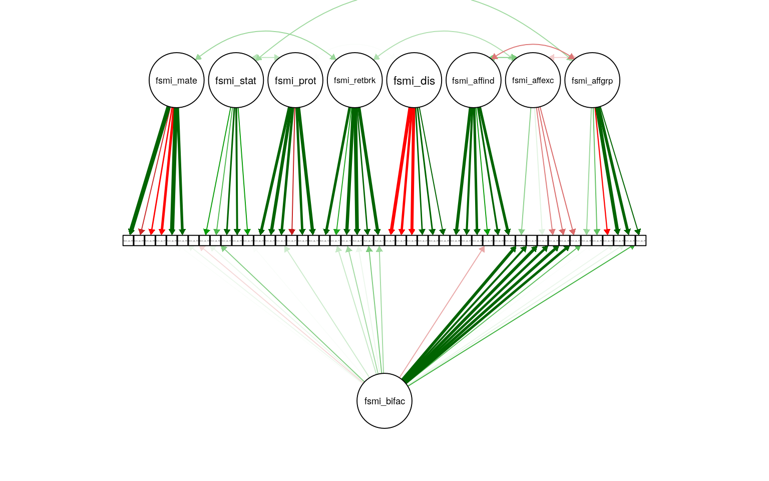
Figure 1: FSMI CFA with method bifactor. Path weight reflects standardized loading strength, with minimum cuttoff for showing path set at .20, and maximum weight at .90 (apparent for several mate-seeking items). Residual and means not shown.
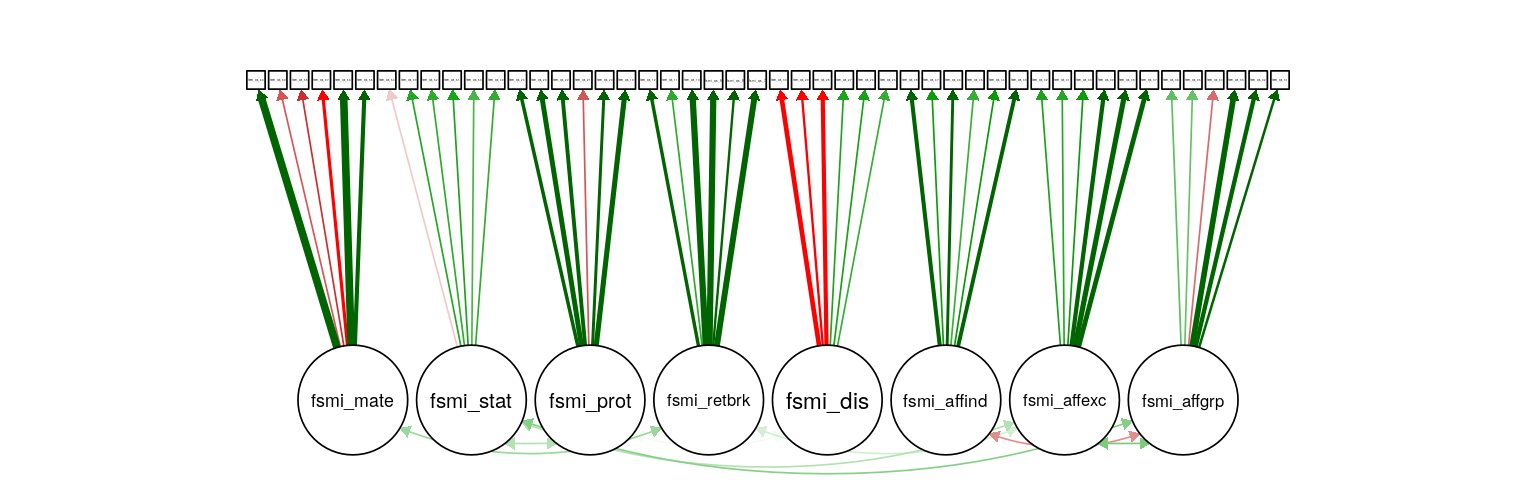
Figure 2: FSMI CFA. Path weight reflects standardized loading strength, with minimum cuttoff for showing path set at .20, and maximum weight at .90 (apparent for several mate-seeking items). Residual and means not shown.
The two factor structures are shown above.
FSMI Discussion
The factor model, fit to all but three of the original scale’s factors (child-care, care for family, general mate retention; N = 225) shows somewhat reasonable, but not great, fit (RMSEA = 0.064, \(\hat\gamma\) = 0.846). This deviates from the results reported by Neel and colleagues (2015), where each factor, or set of related factors, was tested independently. A parallel scree plot analysis (psych package version 1.9.12.31) suggested 8 factors, with all item loadings dominant on expected factors. There is some evidence that including a factor that accounts for an overall method factor improve model fit. Adding such a method bifactor improved the fit somewhat (RMSEA = 0.055, \(\hat\gamma\) = 0.888). Model comparison substantially favors the less parsimonious model that includes the method bifactor (\(\Delta\)AIC = 251, \(\Delta\)BIC = 87, \(\Delta\)Df = 48). Although this bifactor does improve fit across all factors, it does not load strongly on either status or mate-seeking, so I do not account for in in analyses below.
#> $fsmi_cfa_matestat_gender
#>       rmsea         mfi    gammaHat adjGammaHat         AIC
#>      0.0638      0.8976      0.9651      0.9486   9380.3014
#>
#> $fsmi_cfa_matestat_gender_metric
#>       rmsea         mfi    gammaHat adjGammaHat         AIC
#>      0.0593      0.9029      0.9669      0.9555   9367.6660
#>
#> $fsmi_cfa_matestat_gender_metric_cor
#>       rmsea         mfi    gammaHat adjGammaHat         AIC
#>      0.0572      0.9074      0.9685      0.9587   9362.4784
#>
#> $delta1
#>       rmsea         mfi    gammaHat adjGammaHat         AIC
#>     -0.0045      0.0053      0.0018      0.0069    -12.6354
#>
#> $delta2
#>       rmsea         mfi    gammaHat adjGammaHat         AIC
#>     -0.0022      0.0044      0.0015      0.0031     -5.1877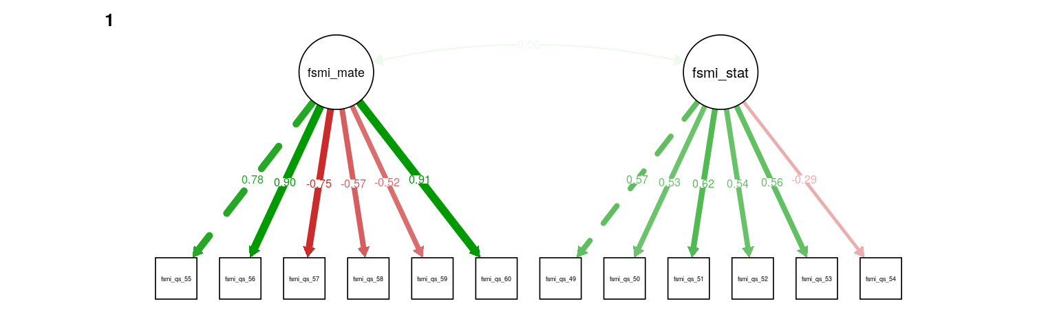
Figure 3: FSMI mate-seeking & status CFA. Path weights and labels reflect standardized loading strength. Residuals, exogenous variances, and means not shown.
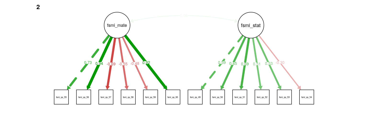
Figure 4: FSMI mate-seeking & status CFA. Path weights and labels reflect standardized loading strength. Residuals, exogenous variances, and means not shown.
A CFA for mate-seeking and status factors fit well (RMSEA = 0.064, \(\hat\gamma\) = 0.967), with the two factors showing a small, positive, non-significant correlation (\(r = 0.06, 0.06, Z = 0.69, 0.69\)). Note that item 54, “I do not worry very much about losing status” has a particularly low loading on the status factor (standardized loading = -0.29, -0.3).
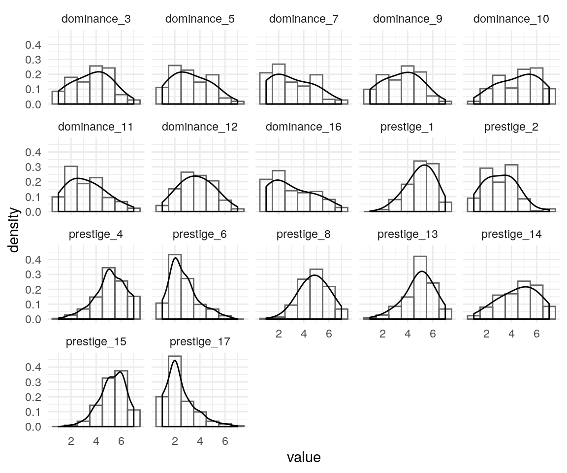
Dominance and Prestige
Measurement invariance
#> $dnp_cfa_gender
#> rmsea mfi gammaHat adjGammaHat AIC
#> 0.0967 0.5757 0.8846 0.8503 12162.9000
#>
#> $dnp_cfa_gender_metric
#> rmsea mfi gammaHat adjGammaHat AIC
#> 0.0965 0.5574 0.8786 0.8520 12162.4116
#>
#> $dnp_cfa_gender_partmetric
#> rmsea mfi gammaHat adjGammaHat AIC
#> 0.0956 0.5649 0.8811 0.8544 12157.4140
#>
#> $dnp_cfa_gender_partmetric_cor
#> rmsea mfi gammaHat adjGammaHat AIC
#> 0.0949 0.5659 0.8814 0.8566 12153.5625
#>
#> $delta1
#> rmsea mfi gammaHat adjGammaHat AIC
#> -0.0002 -0.0183 -0.0060 0.0017 -0.4883
#>
#> $delta2
#> rmsea mfi gammaHat adjGammaHat AIC
#> -0.0011 -0.0108 -0.0035 0.0041 -5.4860
#>
#> $delta3
#> rmsea mfi gammaHat adjGammaHat AIC
#> -0.0007 0.0011 0.0003 0.0021 -3.8515
#> Chi-Squared Difference Test
#>
#> Df AIC BIC Chisq Chisq diff Df diff Pr(>Chisq)
#> dnp_cfa_gender 236 12163 12518 483.37
#> dnp_cfa_gender_partmetric 250 12157 12464 505.88 22.514 14 0.06865
#>
#> dnp_cfa_gender
#> dnp_cfa_gender_partmetric .
#> ---
#> Signif. codes: 0 '***' 0.001 '**' 0.01 '*' 0.05 '.' 0.1 ' ' 1
#> [1] 224
#> [1] 0.095
#> [1] 0.57
#> [1] 0.881
#> $`1`
#> dmnnc_ prstg_
#> dominance_score 1.000
#> prestige_score 0.232 1.000
#>
#> $`0`
#> dmnnc_ prstg_
#> dominance_score 1.000
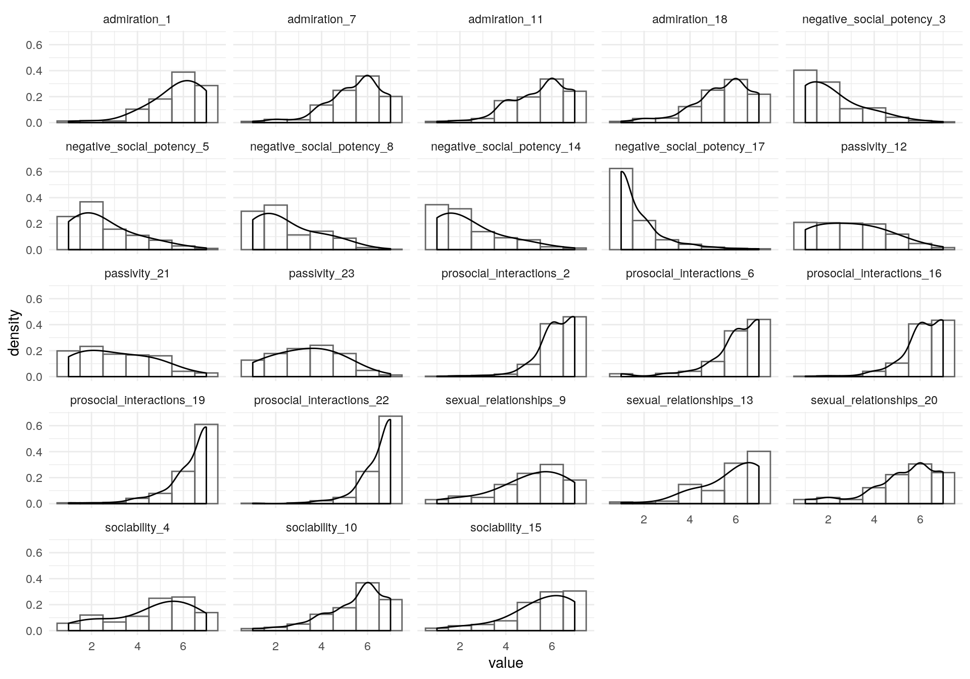
#> prestige_score 0.232 1.000K-SRQ
Measurement invariance
#> $ksrq_cfa
#>        rmsea          mfi     gammaHat  adjGammaHat          AIC
#> 9.289217e-02 7.752621e-01 9.273648e-01 8.879694e-01 1.321388e+04
#>
#> $ksrq_cfa_metric
#>        rmsea          mfi     gammaHat  adjGammaHat          AIC
#> 9.206468e-02 7.664916e-01 9.243639e-01 8.903125e-01 1.320614e+04
#>
#> $ksrq_cfa_metric_full
#>        rmsea          mfi     gammaHat  adjGammaHat          AIC
#> 9.580174e-02 7.395408e-01 9.150481e-01 8.824240e-01 1.321698e+04
#>
#> $ksrq_cfa_metric_cov
#>        rmsea          mfi     gammaHat  adjGammaHat          AIC
#> 9.179351e-02 7.438135e-01 9.165347e-01 8.918813e-01 1.319530e+04
#>
#> $ksrq_cfa_gender
#>        rmsea          mfi     gammaHat  adjGammaHat          AIC
#> 7.065038e-02 8.630794e-01 9.566565e-01 9.331482e-01 1.320130e+04
#>
#> $ksrq_cfa_gender_metric
#>        rmsea          mfi     gammaHat  adjGammaHat          AIC
#> 7.200891e-02 8.526147e-01 9.532336e-01 9.308010e-01 1.320408e+04
#>
#> $delta1
#>         rmsea           mfi      gammaHat   adjGammaHat           AIC
#> -0.0008274881 -0.0087704481 -0.0030009008  0.0023431539 -7.7412448775
#>
#> $delta1a
#>        rmsea          mfi     gammaHat  adjGammaHat          AIC
#>  0.002909573 -0.035721295 -0.012316654 -0.005545380  3.095549704
#>
#> $delta2
#>         rmsea           mfi      gammaHat   adjGammaHat           AIC
#> -2.711699e-04 -2.267811e-02 -7.829127e-03  1.568762e-03 -1.083868e+01
#>
#> $delta_gender
#>        rmsea          mfi     gammaHat  adjGammaHat          AIC
#>  0.001358531 -0.010464673 -0.003422892 -0.002347214  2.782907013
#> Chi-Squared Difference Test
#>
#>                  Df   AIC   BIC  Chisq Chisq diff Df diff Pr(>Chisq)
#> ksrq_cfa        236 13214 13892 398.41
#> ksrq_cfa_metric 251 13206 13827 420.66     22.259      15     0.1012
#> Chi-Squared Difference Test
#>
#>                      Df   AIC   BIC  Chisq Chisq diff Df diff Pr(>Chisq)
#> ksrq_cfa_metric     251 13206 13827 420.66
#> ksrq_cfa_metric_cov 281 13195 13704 469.83     49.161      30    0.01513 *
#> ---
#> Signif. codes:  0 '***' 0.001 '**' 0.01 '*' 0.05 '.' 0.1 ' ' 1
#>                            k_srq_d k_srq_p k_sr__ k_srq_s
#> k_srq_admiration            0.000
#> k_srq_passivity             0.009   0.000
#> k_srq_sexual_relationships -0.023   0.014   0.000
#> k_srq_sociability           0.014   0.016  -0.002  0.000
A CFA for the four K-SRQ factors was tested for metric invariance across samples by comparing a model with loadings constrained to equality to one with loadings free to vary across the four groups. This resulted in considerably worse model fit as determined by a change in the MFI > .01. Loading constraints were removed from four items (“I like it if others looks up to me”, “I like being a member of a group/club”, “I like kissing”, “I like flirting”) that load onto Admiration, Sociability, and Sexual Relationships, respectively. This resulted in adequately small fit differences between the unconstrained and invariant models (\(\Delta\)RMSEA = -0.00083, \(\Delta\)MFI = -0.009, \(\Delta\hat{\gamma}\) = -0.003). The final model showed somewhat poor fit (\(\text{N}_{\text{total}}\) = 319, RMSEA = 0.09, MFI = 0.77, \(\hat\gamma\) = 0.924).
Models with and without constraintes between latent variances and covariances were compared using the Akaike information criterion (AIC). Constraining equivalent latent covariance structures across groups resulted in lower AIC (\(\Delta\text{AIC} = -11\)). Loadings without constraints across groups do not contribute to this comparison, so the magnitude of correlations was compared across the metric invariant and unconstrained models (while mainting the constraint of covariance across groups). The differences in correlations were in the range r = [-0.02, 0.02], indicating very low sensitivity the observed measurement invariance. To maintain content coverage (Borsboom, 2006), the unconstrained model is used, though sensitivity to constraints on the four non-invariant loadings is assessed again. Correlations among the Admiration, Sociability, and Sexual Relationships subscales were all high (r = [.67,.84]). Correlations of Passivity with these three subscales was generally low, but positive (r = [.07, .21]; see Table ??? for all latent variable correlations).
Misc
#> lavaan 0.6-5 ended normally after 218 iterations
#>
#> Estimator ML
#> Optimization method NLMINB
#> Number of free parameters 180
#>
#> Number of observations per group: Used Total
#> yads_online 138 145
#> yads 83 84
#> TDS2 65 65
#> TDS1 33 39
#> Number of missing patterns per group:
#> yads_online 5
#> yads 3
#> TDS2 3
#> TDS1 2
#>
#> Model Test User Model:
#>
#> Test statistic 398.406
#> Degrees of freedom 236
#> P-value (Chi-square) 0.000
#> Test statistic for each group:
#> yads_online 82.868
#> yads 100.301
#> TDS2 124.475
#> TDS1 90.761
#>
#> Parameter Estimates:
#>
#> Information Observed
#> Observed information based on Hessian
#> Standard errors Standard
#>
#>
#> Group 1 [yads_online]:
#>
#> Latent Variables:
#> Estimate Std.Err z-value P(>|z|) Std.lv
#> k_srq_admiration =~
#> K_SRQ_1 1.000 0.984
#> K_SRQ_7 0.947 0.097 9.737 0.000 0.931
#> K_SRQ_11 0.975 0.098 9.970 0.000 0.959
#> K_SRQ_18 1.027 0.108 9.510 0.000 1.010
#> k_srq_passivity =~
#> K_SRQ_12 1.000 1.065
#> K_SRQ_21 1.214 0.185 6.569 0.000 1.293
#> K_SRQ_23 0.957 0.136 7.037 0.000 1.019
#> k_srq_sexual_relationships =~
#> K_SRQ_9 1.000 1.007
#> K_SRQ_13 0.944 0.140 6.759 0.000 0.951
#> K_SRQ_20 1.064 0.163 6.527 0.000 1.071
#> k_srq_sociability =~
#> K_SRQ_4 1.000 0.938
#> K_SRQ_10 1.082 0.191 5.670 0.000 1.014
#> K_SRQ_15 1.063 0.197 5.387 0.000 0.997
#> Std.all
#>
#> 0.791
#> 0.797
#> 0.809
#> 0.775
#>
#> 0.727
#> 0.824
#> 0.696
#>
#> 0.660
#> 0.732
#> 0.705
#>
#> 0.524
#> 0.762
#> 0.683
#>
#> Covariances:
#> Estimate Std.Err z-value P(>|z|) Std.lv
#> k_srq_admiration ~~
#> k_srq_passivty 0.179 0.109 1.636 0.102 0.171
#> k_srq_sxl_rltn 0.776 0.155 5.014 0.000 0.784
#> k_srq_sociblty 0.795 0.169 4.691 0.000 0.862
#> k_srq_passivity ~~
#> k_srq_sxl_rltn 0.127 0.119 1.065 0.287 0.118
#> k_srq_sociblty 0.254 0.120 2.125 0.034 0.254
#> k_srq_sexual_relationships ~~
#> k_srq_sociblty 0.846 0.203 4.169 0.000 0.896
#> Std.all
#>
#> 0.171
#> 0.784
#> 0.862
#>
#> 0.118
#> 0.254
#>
#> 0.896
#>
#> Intercepts:
#> Estimate Std.Err z-value P(>|z|) Std.lv Std.all
#> .K_SRQ_1 5.580 0.106 52.683 0.000 5.580 4.485
#> .K_SRQ_7 5.377 0.099 54.058 0.000 5.377 4.602
#> .K_SRQ_11 5.326 0.101 52.726 0.000 5.326 4.488
#> .K_SRQ_18 5.310 0.111 47.754 0.000 5.310 4.072
#> .K_SRQ_12 2.884 0.125 23.128 0.000 2.884 1.969
#> .K_SRQ_21 3.283 0.134 24.568 0.000 3.283 2.091
#> .K_SRQ_23 3.454 0.126 27.495 0.000 3.454 2.357
#> .K_SRQ_9 5.239 0.130 40.347 0.000 5.239 3.435
#> .K_SRQ_13 5.949 0.111 53.827 0.000 5.949 4.582
#> .K_SRQ_20 5.377 0.129 41.583 0.000 5.377 3.540
#> .K_SRQ_4 4.789 0.153 31.296 0.000 4.789 2.679
#> .K_SRQ_10 5.471 0.113 48.296 0.000 5.471 4.111
#> .K_SRQ_15 5.457 0.124 43.898 0.000 5.457 3.737
#> k_srq_admiratn 0.000 0.000 0.000
#> k_srq_passivty 0.000 0.000 0.000
#> k_srq_sxl_rltn 0.000 0.000 0.000
#> k_srq_sociblty 0.000 0.000 0.000
#>
#> Variances:
#> Estimate Std.Err z-value P(>|z|) Std.lv Std.all
#> .K_SRQ_1 0.580 0.089 6.543 0.000 0.580 0.375
#> .K_SRQ_7 0.498 0.077 6.492 0.000 0.498 0.365
#> .K_SRQ_11 0.488 0.077 6.329 0.000 0.488 0.346
#> .K_SRQ_18 0.679 0.101 6.737 0.000 0.679 0.400
#> .K_SRQ_12 1.011 0.187 5.394 0.000 1.011 0.471
#> .K_SRQ_21 0.793 0.235 3.377 0.001 0.793 0.322
#> .K_SRQ_23 1.108 0.187 5.933 0.000 1.108 0.516
#> .K_SRQ_9 1.314 0.190 6.922 0.000 1.314 0.565
#> .K_SRQ_13 0.782 0.130 5.997 0.000 0.782 0.464
#> .K_SRQ_20 1.161 0.180 6.445 0.000 1.161 0.503
#> .K_SRQ_4 2.317 0.312 7.432 0.000 2.317 0.725
#> .K_SRQ_10 0.742 0.126 5.905 0.000 0.742 0.419
#> .K_SRQ_15 1.138 0.163 6.997 0.000 1.138 0.534
#> k_srq_admiratn 0.968 0.181 5.340 0.000 1.000 1.000
#> k_srq_passivty 1.135 0.269 4.222 0.000 1.000 1.000
#> k_srq_sxl_rltn 1.013 0.254 3.990 0.000 1.000 1.000
#> k_srq_sociblty 0.879 0.299 2.936 0.003 1.000 1.000
#>
#>
#> Group 2 [yads]:
#>
#> Latent Variables:
#> Estimate Std.Err z-value P(>|z|) Std.lv
#> k_srq_admiration =~
#> K_SRQ_1 1.000 0.973
#> K_SRQ_7 0.816 0.122 6.695 0.000 0.794
#> K_SRQ_11 1.164 0.148 7.846 0.000 1.133
#> K_SRQ_18 0.896 0.144 6.224 0.000 0.871
#> k_srq_passivity =~
#> K_SRQ_12 1.000 1.392
#> K_SRQ_21 0.888 0.191 4.642 0.000 1.236
#> K_SRQ_23 0.499 0.137 3.650 0.000 0.695
#> k_srq_sexual_relationships =~
#> K_SRQ_9 1.000 1.073
#> K_SRQ_13 0.563 0.133 4.237 0.000 0.604
#> K_SRQ_20 1.193 0.189 6.303 0.000 1.281
#> k_srq_sociability =~
#> K_SRQ_4 1.000 0.694
#> K_SRQ_10 0.485 0.224 2.169 0.030 0.337
#> K_SRQ_15 1.545 0.530 2.917 0.004 1.073
#> Std.all
#>
#> 0.813
#> 0.714
#> 0.847
#> 0.674
#>
#> 0.915
#> 0.749
#> 0.483
#>
#> 0.769
#> 0.622
#> 0.886
#>
#> 0.406
#> 0.346
#> 0.728
#>
#> Covariances:
#> Estimate Std.Err z-value P(>|z|) Std.lv
#> k_srq_admiration ~~
#> k_srq_passivty 0.236 0.177 1.328 0.184 0.174
#> k_srq_sxl_rltn 0.498 0.172 2.903 0.004 0.477
#> k_srq_sociblty 0.491 0.172 2.853 0.004 0.727
#> k_srq_passivity ~~
#> k_srq_sxl_rltn 0.122 0.195 0.624 0.533 0.081
#> k_srq_sociblty 0.263 0.170 1.543 0.123 0.272
#> k_srq_sexual_relationships ~~
#> k_srq_sociblty 0.538 0.229 2.355 0.019 0.722
#> Std.all
#>
#> 0.174
#> 0.477
#> 0.727
#>
#> 0.081
#> 0.272
#>
#> 0.722
#>
#> Intercepts:
#> Estimate Std.Err z-value P(>|z|) Std.lv Std.all
#> .K_SRQ_1 5.651 0.131 43.017 0.000 5.651 4.722
#> .K_SRQ_7 5.533 0.122 45.176 0.000 5.533 4.976
#> .K_SRQ_11 5.337 0.147 36.346 0.000 5.337 3.990
#> .K_SRQ_18 5.337 0.142 37.635 0.000 5.337 4.131
#> .K_SRQ_12 3.181 0.167 19.038 0.000 3.181 2.090
#> .K_SRQ_21 3.217 0.181 17.757 0.000 3.217 1.949
#> .K_SRQ_23 3.422 0.158 21.640 0.000 3.422 2.375
#> .K_SRQ_9 5.151 0.172 29.990 0.000 5.151 3.691
#> .K_SRQ_13 6.145 0.107 57.648 0.000 6.145 6.328
#> .K_SRQ_20 5.373 0.159 33.867 0.000 5.373 3.717
#> .K_SRQ_4 4.940 0.188 26.318 0.000 4.940 2.889
#> .K_SRQ_10 5.916 0.107 55.449 0.000 5.916 6.086
#> .K_SRQ_15 5.675 0.162 35.085 0.000 5.675 3.851
#> k_srq_admiratn 0.000 0.000 0.000
#> k_srq_passivty 0.000 0.000 0.000
#> k_srq_sxl_rltn 0.000 0.000 0.000
#> k_srq_sociblty 0.000 0.000 0.000
#>
#> Variances:
#> Estimate Std.Err z-value P(>|z|) Std.lv Std.all
#> .K_SRQ_1 0.486 0.111 4.391 0.000 0.486 0.339
#> .K_SRQ_7 0.605 0.113 5.372 0.000 0.605 0.490
#> .K_SRQ_11 0.506 0.132 3.829 0.000 0.506 0.283
#> .K_SRQ_18 0.910 0.162 5.628 0.000 0.910 0.545
#> .K_SRQ_12 0.378 0.374 1.012 0.312 0.378 0.163
#> .K_SRQ_21 1.197 0.346 3.455 0.001 1.197 0.439
#> .K_SRQ_23 1.592 0.267 5.963 0.000 1.592 0.767
#> .K_SRQ_9 0.796 0.200 3.989 0.000 0.796 0.409
#> .K_SRQ_13 0.578 0.117 4.945 0.000 0.578 0.613
#> .K_SRQ_20 0.449 0.274 1.640 0.101 0.449 0.215
#> .K_SRQ_4 2.442 0.422 5.792 0.000 2.442 0.835
#> .K_SRQ_10 0.831 0.135 6.139 0.000 0.831 0.880
#> .K_SRQ_15 1.021 0.308 3.310 0.001 1.021 0.470
#> k_srq_admiratn 0.947 0.224 4.221 0.000 1.000 1.000
#> k_srq_passivty 1.939 0.512 3.786 0.000 1.000 1.000
#> k_srq_sxl_rltn 1.152 0.364 3.167 0.002 1.000 1.000
#> k_srq_sociblty 0.482 0.310 1.552 0.121 1.000 1.000
#>
#>
#> Group 3 [TDS2]:
#>
#> Latent Variables:
#> Estimate Std.Err z-value P(>|z|) Std.lv
#> k_srq_admiration =~
#> K_SRQ_1 1.000 0.577
#> K_SRQ_7 1.148 0.329 3.490 0.000 0.662
#> K_SRQ_11 1.551 0.538 2.883 0.004 0.895
#> K_SRQ_18 1.128 0.336 3.358 0.001 0.651
#> k_srq_passivity =~
#> K_SRQ_12 1.000 1.308
#> K_SRQ_21 0.994 0.250 3.980 0.000 1.300
#> K_SRQ_23 0.819 0.157 5.218 0.000 1.071
#> k_srq_sexual_relationships =~
#> K_SRQ_9 1.000 1.239
#> K_SRQ_13 0.691 0.146 4.742 0.000 0.856
#> K_SRQ_20 1.178 0.190 6.194 0.000 1.459
#> k_srq_sociability =~
#> K_SRQ_4 1.000 1.047
#> K_SRQ_10 0.603 0.267 2.257 0.024 0.631
#> K_SRQ_15 0.881 0.262 3.363 0.001 0.923
#> Std.all
#>
#> 0.568
#> 0.571
#> 0.778
#> 0.575
#>
#> 0.763
#> 0.783
#> 0.742
#>
#> 0.717
#> 0.625
#> 0.918
#>
#> 0.594
#> 0.399
#> 0.667
#>
#> Covariances:
#> Estimate Std.Err z-value P(>|z|) Std.lv
#> k_srq_admiration ~~
#> k_srq_passivty 0.030 0.133 0.224 0.822 0.040
#> k_srq_sxl_rltn 0.401 0.151 2.648 0.008 0.561
#> k_srq_sociblty 0.398 0.151 2.641 0.008 0.659
#> k_srq_passivity ~~
#> k_srq_sxl_rltn 0.648 0.282 2.301 0.021 0.400
#> k_srq_sociblty 0.195 0.275 0.707 0.479 0.142
#> k_srq_sexual_relationships ~~
#> k_srq_sociblty 1.101 0.386 2.855 0.004 0.849
#> Std.all
#>
#> 0.040
#> 0.561
#> 0.659
#>
#> 0.400
#> 0.142
#>
#> 0.849
#>
#> Intercepts:
#> Estimate Std.Err z-value P(>|z|) Std.lv Std.all
#> .K_SRQ_1 6.123 0.126 48.618 0.000 6.123 6.030
#> .K_SRQ_7 5.600 0.144 38.891 0.000 5.600 4.824
#> .K_SRQ_11 6.000 0.143 42.055 0.000 6.000 5.216
#> .K_SRQ_18 5.800 0.141 41.052 0.000 5.800 5.123
#> .K_SRQ_12 3.123 0.213 14.688 0.000 3.123 1.822
#> .K_SRQ_21 2.600 0.207 12.560 0.000 2.600 1.566
#> .K_SRQ_23 3.055 0.180 16.978 0.000 3.055 2.117
#> .K_SRQ_9 5.031 0.214 23.481 0.000 5.031 2.912
#> .K_SRQ_13 5.521 0.171 32.328 0.000 5.521 4.034
#> .K_SRQ_20 5.170 0.198 26.131 0.000 5.170 3.253
#> .K_SRQ_4 4.415 0.219 20.204 0.000 4.415 2.506
#> .K_SRQ_10 5.119 0.198 25.895 0.000 5.119 3.234
#> .K_SRQ_15 5.658 0.173 32.795 0.000 5.658 4.092
#> k_srq_admiratn 0.000 0.000 0.000
#> k_srq_passivty 0.000 0.000 0.000
#> k_srq_sxl_rltn 0.000 0.000 0.000
#> k_srq_sociblty 0.000 0.000 0.000
#>
#> Variances:
#> Estimate Std.Err z-value P(>|z|) Std.lv Std.all
#> .K_SRQ_1 0.698 0.164 4.254 0.000 0.698 0.677
#> .K_SRQ_7 0.909 0.213 4.273 0.000 0.909 0.674
#> .K_SRQ_11 0.523 0.229 2.287 0.022 0.523 0.395
#> .K_SRQ_18 0.859 0.190 4.517 0.000 0.859 0.670
#> .K_SRQ_12 1.228 0.424 2.900 0.004 1.228 0.418
#> .K_SRQ_21 1.068 0.416 2.570 0.010 1.068 0.387
#> .K_SRQ_23 0.935 0.249 3.751 0.000 0.935 0.449
#> .K_SRQ_9 1.450 0.306 4.742 0.000 1.450 0.486
#> .K_SRQ_13 1.141 0.227 5.030 0.000 1.141 0.609
#> .K_SRQ_20 0.397 0.221 1.794 0.073 0.397 0.157
#> .K_SRQ_4 2.008 0.464 4.326 0.000 2.008 0.647
#> .K_SRQ_10 2.107 0.403 5.223 0.000 2.107 0.841
#> .K_SRQ_15 1.061 0.302 3.517 0.000 1.061 0.555
#> k_srq_admiratn 0.333 0.172 1.932 0.053 1.000 1.000
#> k_srq_passivty 1.710 0.594 2.881 0.004 1.000 1.000
#> k_srq_sxl_rltn 1.534 0.488 3.144 0.002 1.000 1.000
#> k_srq_sociblty 1.096 0.514 2.135 0.033 1.000 1.000
#>
#>
#> Group 4 [TDS1]:
#>
#> Latent Variables:
#> Estimate Std.Err z-value P(>|z|) Std.lv
#> k_srq_admiration =~
#> K_SRQ_1 1.000 0.972
#> K_SRQ_7 1.697 0.340 4.986 0.000 1.650
#> K_SRQ_11 1.381 0.269 5.134 0.000 1.342
#> K_SRQ_18 1.238 0.280 4.423 0.000 1.204
#> k_srq_passivity =~
#> K_SRQ_12 1.000 0.657
#> K_SRQ_21 3.508 3.201 1.096 0.273 2.304
#> K_SRQ_23 0.271 0.254 1.069 0.285 0.178
#> k_srq_sexual_relationships =~
#> K_SRQ_9 1.000 0.573
#> K_SRQ_13 2.361 1.012 2.333 0.020 1.352
#> K_SRQ_20 2.640 1.143 2.311 0.021 1.511
#> k_srq_sociability =~
#> K_SRQ_4 1.000 0.966
#> K_SRQ_10 0.605 0.420 1.440 0.150 0.585
#> K_SRQ_15 1.136 0.556 2.044 0.041 1.098
#> Std.all
#>
#> 0.716
#> 0.896
#> 0.926
#> 0.790
#>
#> 0.425
#> 1.520
#> 0.123
#>
#> 0.399
#> 0.890
#> 0.942
#>
#> 0.601
#> 0.350
#> 0.734
#>
#> Covariances:
#> Estimate Std.Err z-value P(>|z|) Std.lv
#> k_srq_admiration ~~
#> k_srq_passivty -0.255 0.279 -0.915 0.360 -0.399
#> k_srq_sxl_rltn 0.411 0.227 1.812 0.070 0.738
#> k_srq_sociblty 0.401 0.266 1.504 0.132 0.426
#> k_srq_passivity ~~
#> k_srq_sxl_rltn -0.099 0.123 -0.807 0.420 -0.264
#> k_srq_sociblty -0.093 0.121 -0.770 0.441 -0.147
#> k_srq_sexual_relationships ~~
#> k_srq_sociblty 0.284 0.198 1.434 0.152 0.513
#> Std.all
#>
#> -0.399
#> 0.738
#> 0.426
#>
#> -0.264
#> -0.147
#>
#> 0.513
#>
#> Intercepts:
#> Estimate Std.Err z-value P(>|z|) Std.lv Std.all
#> .K_SRQ_1 5.818 0.237 24.601 0.000 5.818 4.283
#> .K_SRQ_7 5.394 0.321 16.828 0.000 5.394 2.929
#> .K_SRQ_11 5.667 0.252 22.458 0.000 5.667 3.909
#> .K_SRQ_18 5.492 0.267 20.565 0.000 5.492 3.604
#> .K_SRQ_12 2.909 0.269 10.820 0.000 2.909 1.883
#> .K_SRQ_21 2.939 0.264 11.136 0.000 2.939 1.938
#> .K_SRQ_23 3.364 0.253 13.301 0.000 3.364 2.315
#> .K_SRQ_9 4.939 0.250 19.784 0.000 4.939 3.444
#> .K_SRQ_13 5.424 0.264 20.524 0.000 5.424 3.573
#> .K_SRQ_20 5.303 0.279 18.985 0.000 5.303 3.305
#> .K_SRQ_4 4.333 0.280 15.480 0.000 4.333 2.695
#> .K_SRQ_10 5.152 0.291 17.700 0.000 5.152 3.081
#> .K_SRQ_15 5.394 0.260 20.709 0.000 5.394 3.605
#> k_srq_admiratn 0.000 0.000 0.000
#> k_srq_passivty 0.000 0.000 0.000
#> k_srq_sxl_rltn 0.000 0.000 0.000
#> k_srq_sociblty 0.000 0.000 0.000
#>
#> Variances:
#> Estimate Std.Err z-value P(>|z|) Std.lv Std.all
#> .K_SRQ_1 0.901 0.240 3.746 0.000 0.901 0.488
#> .K_SRQ_7 0.668 0.238 2.810 0.005 0.668 0.197
#> .K_SRQ_11 0.299 0.128 2.333 0.020 0.299 0.142
#> .K_SRQ_18 0.872 0.250 3.488 0.000 0.872 0.376
#> .K_SRQ_12 1.954 0.592 3.303 0.001 1.954 0.819
#> .K_SRQ_21 -3.011 4.294 -0.701 0.483 -3.011 -1.310
#> .K_SRQ_23 2.078 0.509 4.083 0.000 2.078 0.985
#> .K_SRQ_9 1.729 0.434 3.987 0.000 1.729 0.841
#> .K_SRQ_13 0.478 0.204 2.337 0.019 0.478 0.207
#> .K_SRQ_20 0.290 0.229 1.269 0.205 0.290 0.113
#> .K_SRQ_4 1.652 0.591 2.796 0.005 1.652 0.639
#> .K_SRQ_10 2.453 0.677 3.625 0.000 2.453 0.878
#> .K_SRQ_15 1.033 0.614 1.681 0.093 1.033 0.461
#> k_srq_admiratn 0.945 0.407 2.320 0.020 1.000 1.000
#> k_srq_passivty 0.432 0.482 0.896 0.370 1.000 1.000
#> k_srq_sxl_rltn 0.328 0.287 1.144 0.253 1.000 1.000
#> k_srq_sociblty 0.934 0.651 1.435 0.151 1.000 1.000
#> lavaan 0.6-5 ended normally after 49 iterations
#>
#> Estimator ML
#> Optimization method NLMINB
#> Number of free parameters 42
#>
#> Used Total
#> Number of observations 319 334
#> Number of missing patterns 9
#>
#> Model Test User Model:
#> Standard Robust
#> Test Statistic 146.729 118.918
#> Degrees of freedom 62 62
#> P-value (Chi-square) 0.000 0.000
#> Scaling correction factor 1.234
#> for the Yuan-Bentler correction (Mplus variant)
#>
#> Parameter Estimates:
#>
#> Information Observed
#> Observed information based on Hessian
#> Standard errors Robust.huber.white
#>
#> Latent Variables:
#> Estimate Std.Err z-value P(>|z|) Std.lv Std.all
#> ML1 =~
#> K_SRQ_11 1.047 0.069 15.067 0.000 1.047 0.818
#> K_SRQ_18 0.951 0.072 13.135 0.000 0.951 0.727
#> K_SRQ_1 0.926 0.083 11.092 0.000 0.926 0.759
#> K_SRQ_7 0.954 0.070 13.549 0.000 0.954 0.767
#> K_SRQ_10 0.683 0.107 6.393 0.000 0.683 0.496
#> ML2 =~
#> K_SRQ_4 0.936 0.101 9.288 0.000 0.936 0.532
#> K_SRQ_20 1.195 0.086 13.869 0.000 1.195 0.783
#> K_SRQ_13 0.916 0.093 9.904 0.000 0.916 0.711
#> K_SRQ_9 0.992 0.093 10.655 0.000 0.992 0.646
#> K_SRQ_15 0.876 0.093 9.448 0.000 0.876 0.601
#> ML3 =~
#> K_SRQ_12 1.193 0.087 13.644 0.000 1.193 0.771
#> K_SRQ_21 1.263 0.095 13.231 0.000 1.263 0.777
#> K_SRQ_23 0.944 0.082 11.571 0.000 0.944 0.646
#>
#> Covariances:
#> Estimate Std.Err z-value P(>|z|) Std.lv Std.all
#> ML1 ~~
#> ML2 0.662 0.060 11.104 0.000 0.662 0.662
#> ML3 0.048 0.077 0.620 0.535 0.048 0.048
#> ML2 ~~
#> ML3 0.175 0.070 2.489 0.013 0.175 0.175
#>
#> Intercepts:
#> Estimate Std.Err z-value P(>|z|) Std.lv Std.all
#> .K_SRQ_11 5.502 0.072 76.833 0.000 5.502 4.302
#> .K_SRQ_18 5.435 0.073 73.979 0.000 5.435 4.156
#> .K_SRQ_1 5.734 0.068 83.978 0.000 5.734 4.702
#> .K_SRQ_7 5.464 0.070 78.268 0.000 5.464 4.389
#> .K_SRQ_10 5.480 0.077 70.981 0.000 5.480 3.979
#> .K_SRQ_4 4.705 0.099 47.695 0.000 4.705 2.677
#> .K_SRQ_20 5.327 0.086 62.247 0.000 5.327 3.492
#> .K_SRQ_13 5.859 0.072 81.024 0.000 5.859 4.548
#> .K_SRQ_9 5.146 0.088 58.185 0.000 5.146 3.348
#> .K_SRQ_15 5.548 0.082 67.907 0.000 5.548 3.809
#> .K_SRQ_12 3.013 0.087 34.769 0.000 3.013 1.947
#> .K_SRQ_21 3.092 0.091 33.940 0.000 3.092 1.902
#> .K_SRQ_23 3.354 0.082 40.746 0.000 3.354 2.295
#> ML1 0.000 0.000 0.000
#> ML2 0.000 0.000 0.000
#> ML3 0.000 0.000 0.000
#>
#> Variances:
#> Estimate Std.Err z-value P(>|z|) Std.lv Std.all
#> .K_SRQ_11 0.540 0.085 6.355 0.000 0.540 0.330
#> .K_SRQ_18 0.805 0.121 6.638 0.000 0.805 0.471
#> .K_SRQ_1 0.629 0.110 5.710 0.000 0.629 0.423
#> .K_SRQ_7 0.639 0.102 6.242 0.000 0.639 0.412
#> .K_SRQ_10 1.430 0.159 8.998 0.000 1.430 0.754
#> .K_SRQ_4 2.215 0.197 11.243 0.000 2.215 0.717
#> .K_SRQ_20 0.900 0.142 6.344 0.000 0.900 0.387
#> .K_SRQ_13 0.820 0.093 8.838 0.000 0.820 0.494
#> .K_SRQ_9 1.377 0.185 7.439 0.000 1.377 0.583
#> .K_SRQ_15 1.354 0.167 8.098 0.000 1.354 0.638
#> .K_SRQ_12 0.972 0.183 5.306 0.000 0.972 0.406
#> .K_SRQ_21 1.049 0.205 5.106 0.000 1.049 0.397
#> .K_SRQ_23 1.245 0.129 9.643 0.000 1.245 0.583
#> ML1 1.000 1.000 1.000
#> ML2 1.000 1.000 1.000
#> ML3 1.000 1.000 1.000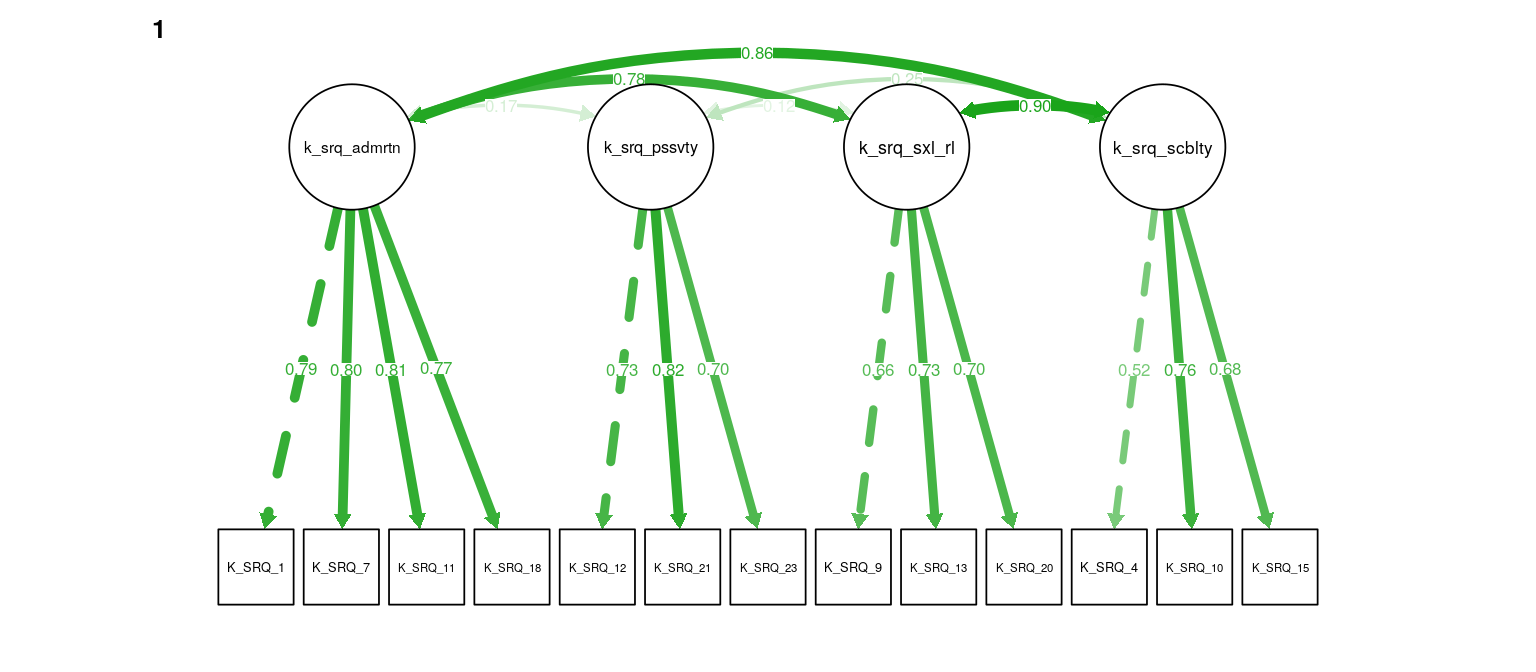
Figure 5: K-SRQ CFA. Path weights and labels reflect standardized loading strength. Residuals, exogenous variances, and means not shown.
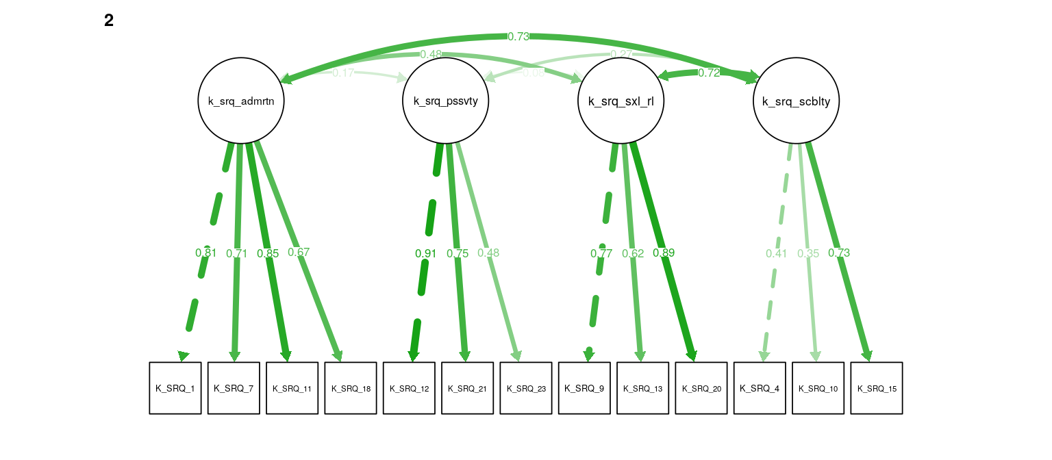
Figure 6: K-SRQ CFA. Path weights and labels reflect standardized loading strength. Residuals, exogenous variances, and means not shown.
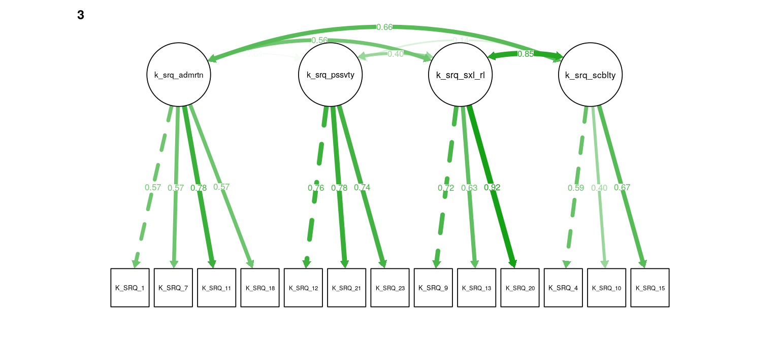
Figure 7: K-SRQ CFA. Path weights and labels reflect standardized loading strength. Residuals, exogenous variances, and means not shown.
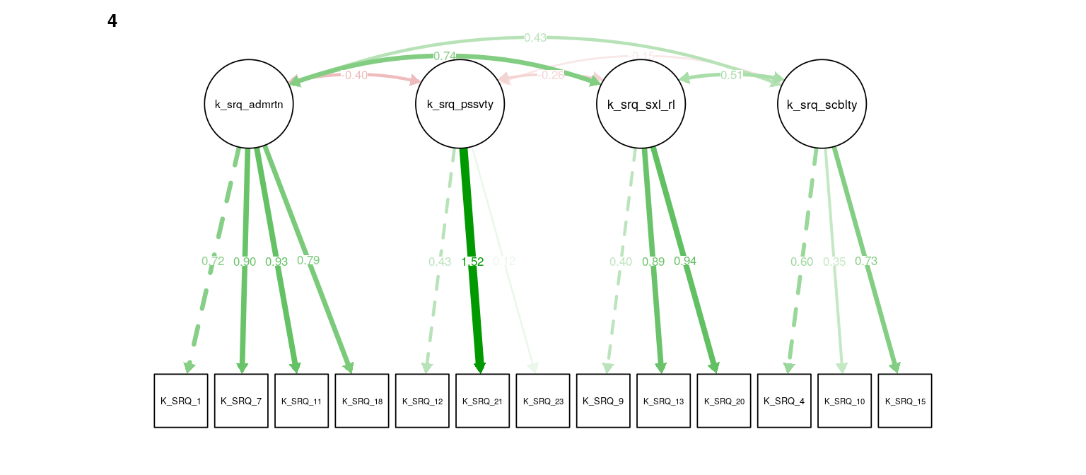
Figure 8: K-SRQ CFA. Path weights and labels reflect standardized loading strength. Residuals, exogenous variances, and means not shown.
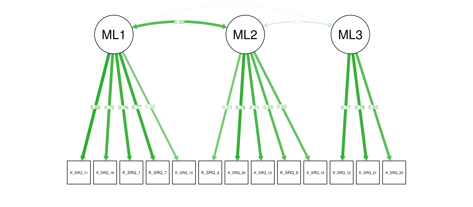
Figure 9: K-SRQ CFA. Path weights and labels reflect standardized loading strength. Residuals, exogenous variances, and means not shown.
#>       rmsea         mfi    gammaHat adjGammaHat
#>    -0.00008    -0.01160    -0.00299     0.00068
#>       rmsea         mfi    gammaHat adjGammaHat
#>     0.00220    -0.02176    -0.00574    -0.00669
#>       rmsea         mfi    gammaHat adjGammaHat
#> -0.00018 0.00109 0.00028 0.00057| lhs | op | rhs | est_rep_1 | est_rep_2 |
|---|---|---|---|---|
| fsmi_mate | ~~ | fsmi_stat | 0.25 [ 0.05, 0.44] | -0.15 [-0.53, 0.24] |
| fsmi_mate | ~~ | k_srq_admiration | 0.35 [ 0.20, 0.50] | -0.31 [-0.68, 0.07] |
| fsmi_mate | ~~ | k_srq_passivity | 0.33 [ 0.18, 0.49] | 0.09 [-0.30, 0.47] |
| fsmi_mate | ~~ | k_srq_sexual_relationships | 0.40 [ 0.23, 0.58] | -0.38 [-0.87, 0.10] |
| fsmi_mate | ~~ | k_srq_sociability | 0.31 [ 0.10, 0.52] | -0.33 [-0.79, 0.14] |
| fsmi_stat | ~~ | k_srq_admiration | 0.69 [ 0.50, 0.88] | 0.53 [ 0.25, 0.82] |
| fsmi_stat | ~~ | k_srq_passivity | -0.06 [-0.29, 0.17] | -0.25 [-0.67, 0.17] |
| fsmi_stat | ~~ | k_srq_sexual_relationships | 0.47 [ 0.25, 0.68] | 0.22 [-0.15, 0.58] |
| fsmi_stat | ~~ | k_srq_sociability | 0.56 [ 0.34, 0.78] | 0.47 [ 0.09, 0.84] |
| k_srq_admiration | ~~ | k_srq_passivity | 0.21 [ 0.04, 0.39] | 0.00 [-0.33, 0.33] |
| k_srq_admiration | ~~ | k_srq_sexual_relationships | 0.66 [ 0.50, 0.82] | 0.81 [ 0.61, 1.02] |
| k_srq_admiration | ~~ | k_srq_sociability | 0.80 [ 0.63, 0.96] | 0.88 [ 0.62, 1.13] |
| k_srq_passivity | ~~ | k_srq_sexual_relationships | 0.08 [-0.09, 0.26] | 0.07 [-0.29, 0.44] |
| k_srq_passivity | ~~ | k_srq_sociability | 0.27 [ 0.07, 0.46] | 0.16 [-0.21, 0.53] |
| k_srq_sexual_relationships | ~~ | k_srq_sociability | 0.80 [ 0.64, 0.96] | 1.05 [ 0.74, 1.35] |
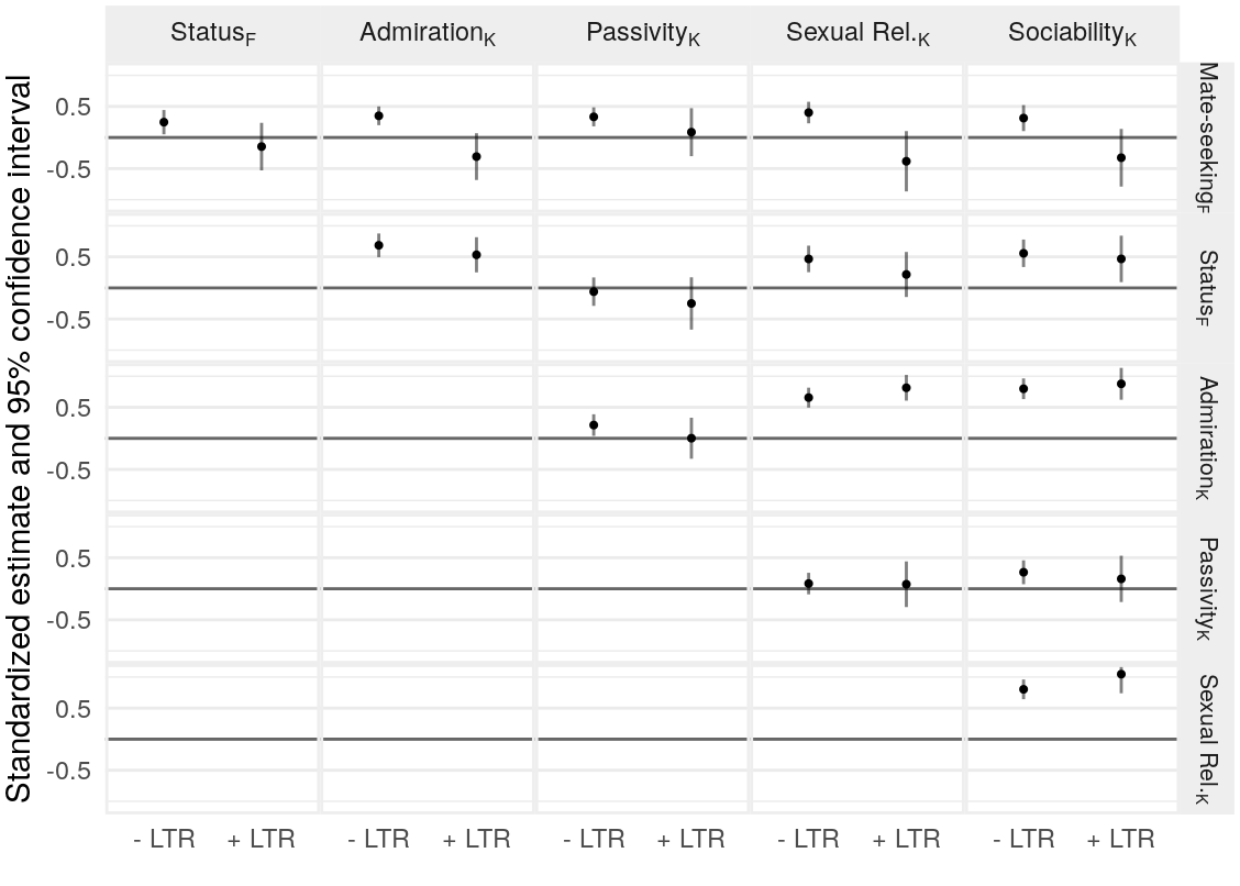
Figure 10: Correlations between FSMI and K-SRQ scales of interest.
K-SRQ and age
#>                                 df         AIC
#> ksrq_cfa_metric_agesem_sample  215 13274.45670
#> ksrq_cfa_metric_agesem         115 13188.22105
#> difference                    -100   -86.23564
#>                                         df         AIC
#> ksrq_cfa_metric_agesem_reginvar         95 13167.34265
#> ksrq_cfa_metric_agesem_reginvar_sample 155 13207.45306
#> difference                              60    40.11041
#>                                         df         AIC
#> ksrq_cfa_metric_agesem_sample          215 13274.45670
#> ksrq_cfa_metric_agesem_reginvar_sample 155 13207.45306
#> difference                             -60   -67.00364
#>                             age_c gender_c age_c2 age_c:gender_c
#> k_srq_admiration           -0.002    0.002  0.000          0.000
#> k_srq_passivity             0.000    0.002  0.000          0.000
#> k_srq_sexual_relationships -0.027   -0.037  0.002         -0.026
#> k_srq_sociability           0.006   -0.013  0.000          0.011
#>                            age_c2:gender_c
#> k_srq_admiration                    -0.001
#> k_srq_passivity                      0.000
#> k_srq_sexual_relationships           0.004
#> k_srq_sociability                    0.003
#>                             age_c gender_c age_c2 age_c:gender_c
#> k_srq_admiration           -0.177   -1.219 -2.401         -0.086
#> k_srq_passivity             0.462    0.245 -1.443          0.755
#> k_srq_sexual_relationships  0.861   -1.277 -2.567         -0.567
#> k_srq_sociability          -0.547    0.022 -2.310         -0.725
#>                            age_c2:gender_c
#> k_srq_admiration                    -0.196
#> k_srq_passivity                     -1.358
#> k_srq_sexual_relationships          -1.592
#> k_srq_sociability                   -1.122
#>                             age_c gender_c age_c2 age_c:gender_c
#> k_srq_admiration           -0.126   -1.226 -2.368         -0.089
#> k_srq_passivity             0.465    0.237 -1.450          0.750
#> k_srq_sexual_relationships  1.448   -1.059 -2.889         -0.129
#> k_srq_sociability          -0.668    0.101 -2.403         -0.901
#>                            age_c2:gender_c
#> k_srq_admiration                    -0.149
#> k_srq_passivity                     -1.360
#> k_srq_sexual_relationships          -1.859
#> k_srq_sociability                   -1.333
#>                             age_c gender_c age_c2 age_c:gender_c
#> k_srq_admiration           -0.051    0.007 -0.033          0.003
#> k_srq_passivity            -0.003    0.008  0.007          0.005
#> k_srq_sexual_relationships -0.587   -0.219  0.323         -0.438
#> k_srq_sociability           0.121   -0.079  0.092          0.175
#>                            age_c2:gender_c
#> k_srq_admiration                    -0.046
#> k_srq_passivity                      0.002
#> k_srq_sexual_relationships           0.266
#> k_srq_sociability                    0.211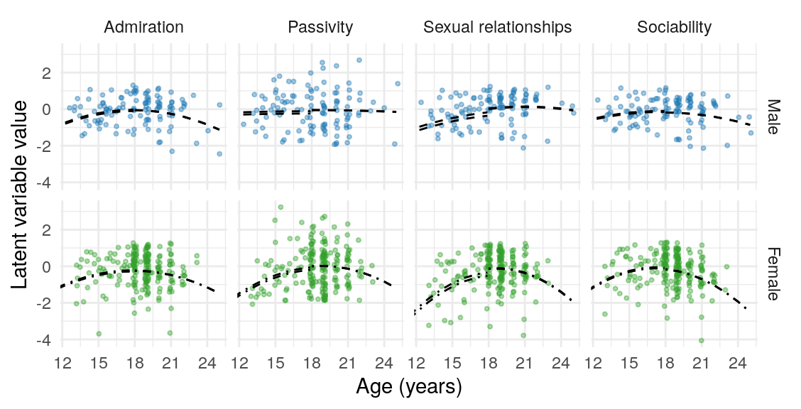
| lhs | op | rhs | block | group | label | est | se | z | pvalue | ci.lower | ci.upper | std.lv | std.all | std.nox |
|---|---|---|---|---|---|---|---|---|---|---|---|---|---|---|
| k_srq_admiration | ~ | age_c | 1 | 1 | .p14. | -0.01 | 0.04 | -0.13 | 0.90 | -0.09 | 0.08 | -0.01 | -0.01 | -0.01 |
| k_srq_admiration | ~ | age_c2 | 1 | 1 | .p15. | -0.02 | 0.01 | -2.37 | 0.02 | -0.04 | 0.00 | -0.03 | -0.13 | -0.03 |
| k_srq_admiration | ~ | gender_c | 1 | 1 | .p16. | -0.18 | 0.15 | -1.23 | 0.22 | -0.48 | 0.11 | -0.20 | -0.09 | -0.20 |
| k_srq_admiration | ~ | age_c:gender_c | 1 | 1 | .p17. | 0.00 | 0.05 | -0.09 | 0.93 | -0.11 | 0.10 | -0.01 | 0.00 | -0.01 |
| k_srq_admiration | ~ | age_c2:gender_c | 1 | 1 | .p18. | 0.00 | 0.02 | -0.15 | 0.88 | -0.04 | 0.03 | 0.00 | -0.01 | 0.00 |
| k_srq_passivity | ~ | age_c | 1 | 1 | .p19. | 0.02 | 0.05 | 0.47 | 0.64 | -0.07 | 0.12 | 0.02 | 0.02 | 0.02 |
| k_srq_passivity | ~ | age_c2 | 1 | 1 | .p20. | -0.02 | 0.01 | -1.45 | 0.15 | -0.04 | 0.01 | -0.01 | -0.07 | -0.01 |
| k_srq_passivity | ~ | gender_c | 1 | 1 | .p21. | 0.05 | 0.22 | 0.24 | 0.81 | -0.38 | 0.49 | 0.04 | 0.02 | 0.04 |
| k_srq_passivity | ~ | age_c:gender_c | 1 | 1 | .p22. | 0.05 | 0.07 | 0.75 | 0.45 | -0.08 | 0.18 | 0.04 | 0.04 | 0.04 |
| k_srq_passivity | ~ | age_c2:gender_c | 1 | 1 | .p23. | -0.03 | 0.02 | -1.36 | 0.17 | -0.07 | 0.01 | -0.02 | -0.08 | -0.02 |
| k_srq_sexual_relationships | ~ | age_c | 1 | 1 | .p24. | 0.07 | 0.05 | 1.45 | 0.15 | -0.02 | 0.16 | 0.07 | 0.09 | 0.07 |
| k_srq_sexual_relationships | ~ | age_c2 | 1 | 1 | .p25. | -0.03 | 0.01 | -2.89 | 0.00 | -0.05 | -0.01 | -0.03 | -0.15 | -0.03 |
| k_srq_sexual_relationships | ~ | gender_c | 1 | 1 | .p26. | -0.16 | 0.15 | -1.06 | 0.29 | -0.45 | 0.14 | -0.17 | -0.07 | -0.17 |
| k_srq_sexual_relationships | ~ | age_c:gender_c | 1 | 1 | .p27. | -0.01 | 0.06 | -0.13 | 0.90 | -0.13 | 0.11 | -0.01 | -0.01 | -0.01 |
| k_srq_sexual_relationships | ~ | age_c2:gender_c | 1 | 1 | .p28. | -0.03 | 0.02 | -1.86 | 0.06 | -0.07 | 0.00 | -0.04 | -0.11 | -0.04 |
| k_srq_sociability | ~ | age_c | 1 | 1 | .p29. | -0.03 | 0.05 | -0.67 | 0.50 | -0.13 | 0.06 | -0.04 | -0.05 | -0.04 |
| k_srq_sociability | ~ | age_c2 | 1 | 1 | .p30. | -0.03 | 0.01 | -2.40 | 0.02 | -0.05 | 0.00 | -0.03 | -0.14 | -0.03 |
| k_srq_sociability | ~ | gender_c | 1 | 1 | .p31. | 0.02 | 0.17 | 0.10 | 0.92 | -0.31 | 0.35 | 0.02 | 0.01 | 0.02 |
| k_srq_sociability | ~ | age_c:gender_c | 1 | 1 | .p32. | -0.05 | 0.06 | -0.90 | 0.37 | -0.17 | 0.06 | -0.06 | -0.05 | -0.06 |
| k_srq_sociability | ~ | age_c2:gender_c | 1 | 1 | .p33. | -0.03 | 0.02 | -1.33 | 0.18 | -0.06 | 0.01 | -0.03 | -0.09 | -0.03 |
| k_srq_admiration | ~ | age_c | 2 | 2 | .p14. | -0.01 | 0.04 | -0.13 | 0.90 | -0.09 | 0.08 | -0.01 | -0.01 | -0.01 |
| k_srq_admiration | ~ | age_c2 | 2 | 2 | .p15. | -0.02 | 0.01 | -2.37 | 0.02 | -0.04 | 0.00 | -0.02 | -0.23 | -0.02 |
| k_srq_admiration | ~ | gender_c | 2 | 2 | .p16. | -0.18 | 0.15 | -1.23 | 0.22 | -0.48 | 0.11 | -0.20 | -0.10 | -0.20 |
| k_srq_admiration | ~ | age_c:gender_c | 2 | 2 | .p17. | 0.00 | 0.05 | -0.09 | 0.93 | -0.11 | 0.10 | -0.01 | -0.01 | -0.01 |
| k_srq_admiration | ~ | age_c2:gender_c | 2 | 2 | .p18. | 0.00 | 0.02 | -0.15 | 0.88 | -0.04 | 0.03 | 0.00 | -0.02 | 0.00 |
| k_srq_passivity | ~ | age_c | 2 | 2 | .p19. | 0.02 | 0.05 | 0.47 | 0.64 | -0.07 | 0.12 | 0.02 | 0.03 | 0.02 |
| k_srq_passivity | ~ | age_c2 | 2 | 2 | .p20. | -0.02 | 0.01 | -1.45 | 0.15 | -0.04 | 0.01 | -0.01 | -0.13 | -0.01 |
| k_srq_passivity | ~ | gender_c | 2 | 2 | .p21. | 0.05 | 0.22 | 0.24 | 0.81 | -0.38 | 0.49 | 0.04 | 0.02 | 0.04 |
| k_srq_passivity | ~ | age_c:gender_c | 2 | 2 | .p22. | 0.05 | 0.07 | 0.75 | 0.45 | -0.08 | 0.18 | 0.04 | 0.05 | 0.04 |
| k_srq_passivity | ~ | age_c2:gender_c | 2 | 2 | .p23. | -0.03 | 0.02 | -1.36 | 0.17 | -0.07 | 0.01 | -0.02 | -0.13 | -0.02 |
| k_srq_sexual_relationships | ~ | age_c | 2 | 2 | .p24. | 0.07 | 0.05 | 1.45 | 0.15 | -0.02 | 0.16 | 0.07 | 0.11 | 0.07 |
| k_srq_sexual_relationships | ~ | age_c2 | 2 | 2 | .p25. | -0.03 | 0.01 | -2.89 | 0.00 | -0.05 | -0.01 | -0.03 | -0.28 | -0.03 |
| k_srq_sexual_relationships | ~ | gender_c | 2 | 2 | .p26. | -0.16 | 0.15 | -1.06 | 0.29 | -0.45 | 0.14 | -0.16 | -0.08 | -0.16 |
| k_srq_sexual_relationships | ~ | age_c:gender_c | 2 | 2 | .p27. | -0.01 | 0.06 | -0.13 | 0.90 | -0.13 | 0.11 | -0.01 | -0.01 | -0.01 |
| k_srq_sexual_relationships | ~ | age_c2:gender_c | 2 | 2 | .p28. | -0.03 | 0.02 | -1.86 | 0.06 | -0.07 | 0.00 | -0.04 | -0.19 | -0.04 |
| k_srq_sociability | ~ | age_c | 2 | 2 | .p29. | -0.03 | 0.05 | -0.67 | 0.50 | -0.13 | 0.06 | -0.04 | -0.06 | -0.04 |
| k_srq_sociability | ~ | age_c2 | 2 | 2 | .p30. | -0.03 | 0.01 | -2.40 | 0.02 | -0.05 | 0.00 | -0.03 | -0.26 | -0.03 |
| k_srq_sociability | ~ | gender_c | 2 | 2 | .p31. | 0.02 | 0.17 | 0.10 | 0.92 | -0.31 | 0.35 | 0.02 | 0.01 | 0.02 |
| k_srq_sociability | ~ | age_c:gender_c | 2 | 2 | .p32. | -0.05 | 0.06 | -0.90 | 0.37 | -0.17 | 0.06 | -0.06 | -0.07 | -0.06 |
| k_srq_sociability | ~ | age_c2:gender_c | 2 | 2 | .p33. | -0.03 | 0.02 | -1.33 | 0.18 | -0.06 | 0.01 | -0.03 | -0.15 | -0.03 |
| k_srq_admiration | ~ | age_c | 3 | 3 | .p14. | -0.01 | 0.04 | -0.13 | 0.90 | -0.09 | 0.08 | -0.01 | -0.01 | -0.01 |
| k_srq_admiration | ~ | age_c2 | 3 | 3 | .p15. | -0.02 | 0.01 | -2.37 | 0.02 | -0.04 | 0.00 | -0.02 | -0.19 | -0.02 |
| k_srq_admiration | ~ | gender_c | 3 | 3 | .p16. | -0.18 | 0.15 | -1.23 | 0.22 | -0.48 | 0.11 | -0.20 | -0.10 | -0.20 |
| k_srq_admiration | ~ | age_c:gender_c | 3 | 3 | .p17. | 0.00 | 0.05 | -0.09 | 0.93 | -0.11 | 0.10 | -0.01 | -0.01 | -0.01 |
| k_srq_admiration | ~ | age_c2:gender_c | 3 | 3 | .p18. | 0.00 | 0.02 | -0.15 | 0.88 | -0.04 | 0.03 | 0.00 | -0.02 | 0.00 |
| k_srq_passivity | ~ | age_c | 3 | 3 | .p19. | 0.02 | 0.05 | 0.47 | 0.64 | -0.07 | 0.12 | 0.02 | 0.03 | 0.02 |
| k_srq_passivity | ~ | age_c2 | 3 | 3 | .p20. | -0.02 | 0.01 | -1.45 | 0.15 | -0.04 | 0.01 | -0.01 | -0.10 | -0.01 |
| k_srq_passivity | ~ | gender_c | 3 | 3 | .p21. | 0.05 | 0.22 | 0.24 | 0.81 | -0.38 | 0.49 | 0.04 | 0.02 | 0.04 |
| k_srq_passivity | ~ | age_c:gender_c | 3 | 3 | .p22. | 0.05 | 0.07 | 0.75 | 0.45 | -0.08 | 0.18 | 0.04 | 0.06 | 0.04 |
| k_srq_passivity | ~ | age_c2:gender_c | 3 | 3 | .p23. | -0.03 | 0.02 | -1.36 | 0.17 | -0.07 | 0.01 | -0.02 | -0.13 | -0.02 |
| k_srq_sexual_relationships | ~ | age_c | 3 | 3 | .p24. | 0.07 | 0.05 | 1.45 | 0.15 | -0.02 | 0.16 | 0.06 | 0.10 | 0.06 |
| k_srq_sexual_relationships | ~ | age_c2 | 3 | 3 | .p25. | -0.03 | 0.01 | -2.89 | 0.00 | -0.05 | -0.01 | -0.03 | -0.21 | -0.03 |
| k_srq_sexual_relationships | ~ | gender_c | 3 | 3 | .p26. | -0.16 | 0.15 | -1.06 | 0.29 | -0.45 | 0.14 | -0.15 | -0.08 | -0.15 |
| k_srq_sexual_relationships | ~ | age_c:gender_c | 3 | 3 | .p27. | -0.01 | 0.06 | -0.13 | 0.90 | -0.13 | 0.11 | -0.01 | -0.01 | -0.01 |
| k_srq_sexual_relationships | ~ | age_c2:gender_c | 3 | 3 | .p28. | -0.03 | 0.02 | -1.86 | 0.06 | -0.07 | 0.00 | -0.03 | -0.19 | -0.03 |
| k_srq_sociability | ~ | age_c | 3 | 3 | .p29. | -0.03 | 0.05 | -0.67 | 0.50 | -0.13 | 0.06 | -0.04 | -0.06 | -0.04 |
| k_srq_sociability | ~ | age_c2 | 3 | 3 | .p30. | -0.03 | 0.01 | -2.40 | 0.02 | -0.05 | 0.00 | -0.03 | -0.21 | -0.03 |
| k_srq_sociability | ~ | gender_c | 3 | 3 | .p31. | 0.02 | 0.17 | 0.10 | 0.92 | -0.31 | 0.35 | 0.02 | 0.01 | 0.02 |
| k_srq_sociability | ~ | age_c:gender_c | 3 | 3 | .p32. | -0.05 | 0.06 | -0.90 | 0.37 | -0.17 | 0.06 | -0.06 | -0.09 | -0.06 |
| k_srq_sociability | ~ | age_c2:gender_c | 3 | 3 | .p33. | -0.03 | 0.02 | -1.33 | 0.18 | -0.06 | 0.01 | -0.03 | -0.16 | -0.03 |
| k_srq_admiration | ~ | age_c | 4 | 4 | .p14. | -0.01 | 0.04 | -0.13 | 0.90 | -0.09 | 0.08 | -0.01 | -0.01 | -0.01 |
| k_srq_admiration | ~ | age_c2 | 4 | 4 | .p15. | -0.02 | 0.01 | -2.37 | 0.02 | -0.04 | 0.00 | -0.03 | -0.17 | -0.03 |
| k_srq_admiration | ~ | gender_c | 4 | 4 | .p16. | -0.18 | 0.15 | -1.23 | 0.22 | -0.48 | 0.11 | -0.20 | -0.10 | -0.20 |
| k_srq_admiration | ~ | age_c:gender_c | 4 | 4 | .p17. | 0.00 | 0.05 | -0.09 | 0.93 | -0.11 | 0.10 | -0.01 | -0.01 | -0.01 |
| k_srq_admiration | ~ | age_c2:gender_c | 4 | 4 | .p18. | 0.00 | 0.02 | -0.15 | 0.88 | -0.04 | 0.03 | 0.00 | -0.01 | 0.00 |
| k_srq_passivity | ~ | age_c | 4 | 4 | .p19. | 0.02 | 0.05 | 0.47 | 0.64 | -0.07 | 0.12 | 0.02 | 0.03 | 0.02 |
| k_srq_passivity | ~ | age_c2 | 4 | 4 | .p20. | -0.02 | 0.01 | -1.45 | 0.15 | -0.04 | 0.01 | -0.01 | -0.09 | -0.01 |
| k_srq_passivity | ~ | gender_c | 4 | 4 | .p21. | 0.05 | 0.22 | 0.24 | 0.81 | -0.38 | 0.49 | 0.04 | 0.02 | 0.04 |
| k_srq_passivity | ~ | age_c:gender_c | 4 | 4 | .p22. | 0.05 | 0.07 | 0.75 | 0.45 | -0.08 | 0.18 | 0.04 | 0.05 | 0.04 |
| k_srq_passivity | ~ | age_c2:gender_c | 4 | 4 | .p23. | -0.03 | 0.02 | -1.36 | 0.17 | -0.07 | 0.01 | -0.02 | -0.10 | -0.02 |
| k_srq_sexual_relationships | ~ | age_c | 4 | 4 | .p24. | 0.07 | 0.05 | 1.45 | 0.15 | -0.02 | 0.16 | 0.07 | 0.12 | 0.07 |
| k_srq_sexual_relationships | ~ | age_c2 | 4 | 4 | .p25. | -0.03 | 0.01 | -2.89 | 0.00 | -0.05 | -0.01 | -0.03 | -0.20 | -0.03 |
| k_srq_sexual_relationships | ~ | gender_c | 4 | 4 | .p26. | -0.16 | 0.15 | -1.06 | 0.29 | -0.45 | 0.14 | -0.16 | -0.08 | -0.16 |
| k_srq_sexual_relationships | ~ | age_c:gender_c | 4 | 4 | .p27. | -0.01 | 0.06 | -0.13 | 0.90 | -0.13 | 0.11 | -0.01 | -0.01 | -0.01 |
| k_srq_sexual_relationships | ~ | age_c2:gender_c | 4 | 4 | .p28. | -0.03 | 0.02 | -1.86 | 0.06 | -0.07 | 0.00 | -0.03 | -0.15 | -0.03 |
| k_srq_sociability | ~ | age_c | 4 | 4 | .p29. | -0.03 | 0.05 | -0.67 | 0.50 | -0.13 | 0.06 | -0.04 | -0.06 | -0.04 |
| k_srq_sociability | ~ | age_c2 | 4 | 4 | .p30. | -0.03 | 0.01 | -2.40 | 0.02 | -0.05 | 0.00 | -0.03 | -0.19 | -0.03 |
| k_srq_sociability | ~ | gender_c | 4 | 4 | .p31. | 0.02 | 0.17 | 0.10 | 0.92 | -0.31 | 0.35 | 0.02 | 0.01 | 0.02 |
| k_srq_sociability | ~ | age_c:gender_c | 4 | 4 | .p32. | -0.05 | 0.06 | -0.90 | 0.37 | -0.17 | 0.06 | -0.06 | -0.07 | -0.06 |
| k_srq_sociability | ~ | age_c2:gender_c | 4 | 4 | .p33. | -0.03 | 0.02 | -1.33 | 0.18 | -0.06 | 0.01 | -0.03 | -0.12 | -0.03 |
| K-SRQ factor | Sample | \(\text{Age}\) | \(\text{Age}\times\text{Gender}\) | \(\text{Age}^2\) | \(\text{Age}^2\times\text{Gender}\) |
|---|---|---|---|---|---|
| Admiration | FCA | -0.01 [-0.17, 0.15] | -0.01 [-0.14, 0.13] | -0.17 [-0.31, -0.03] | -0.01 [-0.19, 0.16] |
| CA | -0.01 [-0.15, 0.13] | -0.01 [-0.17, 0.16] | -0.19 [-0.34, -0.04] | -0.02 [-0.25, 0.21] | |
| CSYA | -0.01 [-0.15, 0.13] | -0.01 [-0.14, 0.13] | -0.23 [-0.41, -0.05] | -0.02 [-0.23, 0.20] | |
| CSYA-O | -0.01 [-0.12, 0.11] | -0.00 [-0.11, 0.10] | -0.13 [-0.24, -0.02] | -0.01 [-0.14, 0.12] | |
| Passivity | FCA | 0.03 [-0.11, 0.17] | 0.05 [-0.08, 0.17] | -0.09 [-0.21, 0.03] | -0.10 [-0.25, 0.05] |
| CA | 0.03 [-0.09, 0.15] | 0.06 [-0.09, 0.21] | -0.10 [-0.24, 0.03] | -0.13 [-0.33, 0.06] | |
| CSYA | 0.03 [-0.10, 0.16] | 0.05 [-0.08, 0.17] | -0.13 [-0.30, 0.04] | -0.13 [-0.31, 0.06] | |
| CSYA-O | 0.02 [-0.08, 0.13] | 0.04 [-0.06, 0.14] | -0.07 [-0.17, 0.02] | -0.08 [-0.19, 0.03] | |
| Sexual Relationships | FCA | 0.12 [-0.04, 0.27] | -0.01 [-0.15, 0.13] | -0.20 [-0.32, -0.08] | -0.15 [-0.30, 0.00] |
| CA | 0.10 [-0.03, 0.23] | -0.01 [-0.18, 0.16] | -0.21 [-0.34, -0.09] | -0.19 [-0.37, -0.00] | |
| CSYA | 0.11 [-0.04, 0.25] | -0.01 [-0.15, 0.13] | -0.28 [-0.45, -0.10] | -0.19 [-0.38, 0.00] | |
| CSYA-O | 0.09 [-0.03, 0.21] | -0.01 [-0.12, 0.11] | -0.15 [-0.26, -0.05] | -0.11 [-0.23, 0.00] | |
| Sociability | FCA | -0.06 [-0.25, 0.12] | -0.07 [-0.22, 0.08] | -0.19 [-0.34, -0.04] | -0.12 [-0.30, 0.06] |
| CA | -0.06 [-0.22, 0.11] | -0.09 [-0.27, 0.10] | -0.21 [-0.38, -0.05] | -0.16 [-0.39, 0.07] | |
| CSYA | -0.06 [-0.22, 0.10] | -0.07 [-0.21, 0.08] | -0.26 [-0.45, -0.06] | -0.15 [-0.36, 0.07] | |
| CSYA-O | -0.05 [-0.18, 0.09] | -0.05 [-0.17, 0.06] | -0.14 [-0.25, -0.03] | -0.09 [-0.22, 0.04] |
K-SRQ PDS
#>                                         df         AIC
#> ksrq_cfa_metric_pdssem_sample          215 13037.36089
#> ksrq_cfa_metric_pdssem_reginvar_sample 155 12979.41555
#> difference                             -60   -57.94535
#>                                         df         AIC
#> ksrq_cfa_metric_pdssem_sample          215 13037.36089
#> ksrq_cfa_metric_pdssem_reginvar_sample 155 12979.41555
#> difference                             -60   -57.94535
#>                            pds_c gender_c pds_c2 pds_c:gender_c pds_c2:gender_c
#> k_srq_admiration           0.661   -0.464 -0.185          0.945          -0.380
#> k_srq_passivity            0.456   -0.517 -0.388          0.909          -0.395
#> k_srq_sexual_relationships 0.812   -0.667 -0.348          0.925          -0.423
#> k_srq_sociability          0.883   -0.883 -0.214          1.388          -0.334
#>                                    pds_c      gender_c        pds_c2
#> k_srq_admiration            4.589433e-03 -0.0039546306  1.164152e-04
#> k_srq_passivity            -2.544921e-05  0.0002948243 -5.584834e-06
#> k_srq_sexual_relationships -2.753713e-02  0.0045892229  8.910481e-03
#> k_srq_sociability          -2.745947e-02  0.0009030445  2.879362e-02
#>                            pds_c:gender_c pds_c2:gender_c
#> k_srq_admiration             0.0004830186   -0.0005093284
#> k_srq_passivity              0.0011816081   -0.0004068115
#> k_srq_sexual_relationships  -0.0153083900    0.0048745359
#> k_srq_sociability           -0.0445051287    0.0475490516
#>                            pds_c gender_c pds_c2 pds_c:gender_c pds_c2:gender_c
#> k_srq_admiration           2.716   -2.550 -0.925          2.039          -0.868
#> k_srq_passivity            1.578   -1.393 -1.305          1.662          -0.692
#> k_srq_sexual_relationships 2.920   -2.902 -1.407          1.682          -0.846
#> k_srq_sociability          3.524   -3.100 -1.002          2.722          -0.746
#>                            pds_c gender_c pds_c2 pds_c:gender_c pds_c2:gender_c
#> k_srq_admiration           2.644   -2.496 -0.920          2.027          -0.855
#> k_srq_passivity            1.578   -1.396 -1.304          1.653          -0.689
#> k_srq_sexual_relationships 3.235   -2.837 -1.523          1.802          -0.871
#> k_srq_sociability          3.459   -3.100 -1.310          2.782          -1.004
#>                             pds_c gender_c pds_c2 pds_c:gender_c
#> k_srq_admiration            0.072   -0.054 -0.005          0.012
#> k_srq_passivity             0.000    0.003 -0.001          0.009
#> k_srq_sexual_relationships -0.315   -0.066  0.115         -0.121
#> k_srq_sociability           0.065    0.000  0.308         -0.060
#>                            pds_c2:gender_c
#> k_srq_admiration                    -0.014
#> k_srq_passivity                     -0.002
#> k_srq_sexual_relationships           0.024
#> k_srq_sociability                    0.258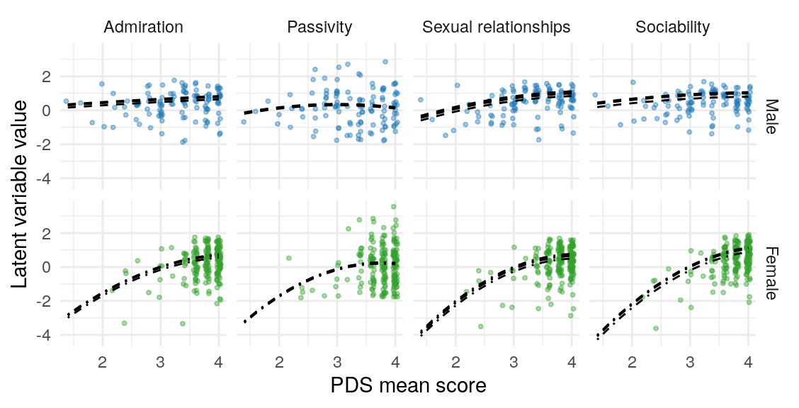
| K-SRQ factor | Sample | \(\text{PDS}\) | \(\text{PDS}\times\text{Gender}\) | \(\text{PDS}^2\) | \(\text{PDS}^2\times\text{Gender}\) |
|---|---|---|---|---|---|
| Admiration | FCA | 0.43 [0.12, 0.74] | 0.28 [0.02, 0.54] | -0.10 [-0.32, 0.12] | -0.14 [-0.44, 0.17] |
| CA | 0.39 [0.13, 0.64] | 0.26 [0.03, 0.48] | -0.09 [-0.28, 0.10] | -0.11 [-0.36, 0.14] | |
| CSYA | 0.19 [0.05, 0.32] | 0.39 [0.03, 0.75] | -0.08 [-0.24, 0.08] | -0.14 [-0.46, 0.18] | |
| CSYA-O | 0.26 [0.08, 0.45] | 0.35 [0.03, 0.67] | -0.07 [-0.23, 0.08] | -0.13 [-0.44, 0.17] | |
| Passivity | FCA | 0.24 [-0.06, 0.54] | 0.21 [-0.05, 0.47] | -0.15 [-0.38, 0.08] | -0.11 [-0.43, 0.21] |
| CA | 0.22 [-0.05, 0.49] | 0.20 [-0.04, 0.44] | -0.14 [-0.34, 0.07] | -0.09 [-0.36, 0.17] | |
| CSYA | 0.10 [-0.03, 0.23] | 0.29 [-0.06, 0.65] | -0.11 [-0.28, 0.06] | -0.12 [-0.44, 0.21] | |
| CSYA-O | 0.15 [-0.03, 0.33] | 0.27 [-0.05, 0.59] | -0.11 [-0.27, 0.05] | -0.11 [-0.43, 0.20] | |
| Sexual Relationships | FCA | 0.59 [0.23, 0.96] | 0.27 [-0.03, 0.57] | -0.19 [-0.43, 0.06] | -0.16 [-0.52, 0.20] |
| CA | 0.53 [0.23, 0.82] | 0.24 [-0.01, 0.49] | -0.16 [-0.37, 0.04] | -0.13 [-0.41, 0.16] | |
| CSYA | 0.26 [0.09, 0.42] | 0.38 [-0.04, 0.79] | -0.14 [-0.32, 0.05] | -0.16 [-0.54, 0.21] | |
| CSYA-O | 0.36 [0.15, 0.58] | 0.34 [-0.02, 0.69] | -0.13 [-0.30, 0.04] | -0.15 [-0.50, 0.19] | |
| Sociability | FCA | 0.65 [0.28, 1.03] | 0.46 [0.14, 0.79] | -0.17 [-0.43, 0.09] | -0.19 [-0.55, 0.17] |
| CA | 0.55 [0.29, 0.81] | 0.40 [0.16, 0.63] | -0.14 [-0.35, 0.07] | -0.14 [-0.41, 0.13] | |
| CSYA | 0.28 [0.12, 0.45] | 0.65 [0.19, 1.10] | -0.13 [-0.32, 0.07] | -0.19 [-0.57, 0.18] | |
| CSYA-O | 0.39 [0.19, 0.59] | 0.56 [0.20, 0.93] | -0.12 [-0.29, 0.06] | -0.18 [-0.52, 0.16] |
K-SRQ Discussion
A CFA for four of the K-SRQ factors (admiration, passivity, sexual relationships, and sociability) fit fairly well (RMSEA = 0.093, \(\hat\gamma\) = 0.924). All factors except passivity were strongly inter-correlated, raising doubts about the discriminant validity of the separate factors. A parallel scree plot analysis suggests a 3 factor structure, with one item from the original sociability factor loading on a factor with the admiration items (weakly), and the other two loading with the sexual relationships items. A CFA using this factor structure (with no cross-loadings) demonstrates similar fit to the a priori model (RMSEA = 0.093, \(\hat\gamma\) = 0.924), and with similarly substantial correlations between the former admiration and sexual relationships factors. A 4 factor EFA retains this general structure, while letting the sociability item, which previously loaded with admiration items, dominate its own factor. The new 3-factor structure improves somewhat on the a priori model, but the sexual relationships factor has not become any more interpretable as representing a mate-seeking motivation, per se. Moreover, the sexual relationship factor, as well as its cousin in the 3-factor model both show nominally higher correlations with FSMI status than FSMI mate-seeking. I use the a priori scale throughout.
The items on the FSMI mate-seeking scale ask almost exlusively aboout seaching for a new romantic or sexula partner, while the K-SRQ sexual relationship scale asks about enjoyment of socio-sexual interaction (e.g., kissing, flirting). One would expect that the FSMI mate-seeking and K-SRQ sexual relationship correlation would be different between those who are in long term relationships and those who are not. There is, in fact, a notable difference in the sign of this correlation between people who report being in a long-term relationship than people how report dating, or being single and not dating. In a model where factor loadings have been constrained across group (with minimal difference in fit statistics which is necessary for comparison of factor covariances; \(\Delta\)RMSEA = -0.00008, \(\Delta\)MFI = -0.012, \(\Delta\hat{\gamma}\) = -0.003; Gregorich, 2006), people who are in a long term relationship show a negative correlation between FSMI mate-seeking K-SRQ sexual relationships (Table ??. For people who are not in long-term relationships, there is a positive, significant, correlation between FSMI mate-seeking and the K-SRQ sexual relationships factor. The relation between FSMI status and this same factor is, however, nominally higher regardless of long-term relationship status.
The K-SRQ admiration-derived factor showed reasonably high correlation with FSMI status, although this was not dissimiler in magnitude from the correlation it shows with the K-SRQ sexual relationship factor.
Generally, the three K-SRQ subscales of interest (but not the passivity subscale) all correlate rather highly among themselves. All four K-SRQ subscales (inlcuding passivity) tend to medium to small correlations with FSMI mate-seeking among people not in long-term relationships, and small or negative correlations among those not in long-term relationships. Across both groups, FSMI status shows medium to large correlations to the K-SRQ subscales except for passivity.
Given how differently the K-SRQ sexual relationships factor covaries with other relevant contructs and across groups, it is clear that it is measuring something distinctly from what the FSMI mate seeking factor is measuring. The distinction between the seeking new romantic or sexual partners, and enjoyment of engaging in socio-sexual behavior may be important when examining how these motivational factors relate to risk-taking. Past work has shown that sexual activity (age at first sex, specifically), if it is in the context of a romantic relationshuip, is protective with respect to dellinquency (Harden & Mendle, 2011; Harden, Mendle, Hill, Turkheimer, & Emery, 2007).
Urgency, premeditation, perseverence, sensation seeking
Measurement invariance
#> $uppsp_cfa
#>       rmsea         mfi    gammaHat adjGammaHat         AIC
#>      0.0733      0.0121      0.7692      0.7512  38112.7580
#>
#> $uppsp_cfa_metric
#>       rmsea         mfi    gammaHat adjGammaHat         AIC
#>      0.0734      0.0112      0.7658      0.7517  38109.4703
#>
#> $uppsp_cfa_metric_cov
#>       rmsea         mfi    gammaHat adjGammaHat         AIC
#>      0.0733      0.0111      0.7657      0.7526  38096.2964
#>
#> $uppsp_cfa_gender
#>       rmsea         mfi    gammaHat adjGammaHat         AIC
#>      0.0727      0.0130      0.7719      0.7542  38305.7078
#>
#> $uppsp_cfa_gender_metric
#>       rmsea         mfi    gammaHat adjGammaHat         AIC
#>      0.0724      0.0125      0.7705      0.7566  38273.8455
#>
#> $delta1
#>       rmsea         mfi    gammaHat adjGammaHat         AIC
#>      0.0001     -0.0010     -0.0034      0.0004     -3.2877
#>
#> $delta2
#>       rmsea         mfi    gammaHat adjGammaHat         AIC
#>     -0.0001      0.0000     -0.0001      0.0010    -13.1740
#>
#> $delta_gender
#>       rmsea         mfi    gammaHat adjGammaHat         AIC
#>     -0.0003     -0.0005     -0.0015      0.0024    -31.8623
#> Chi-Squared Difference Test
#>
#>                    Df   AIC   BIC  Chisq Chisq diff Df diff Pr(>Chisq)
#> uppsp_cfa        3284 38113 39499 5939.4
#> uppsp_cfa_metric 3338 38109 39296 6044.1     104.71      54  4.301e-05 ***
#> ---
#> Signif. codes:  0 '***' 0.001 '**' 0.01 '*' 0.05 '.' 0.1 ' ' 1
#> Chi-Squared Difference Test
#>
#>                        Df   AIC   BIC  Chisq Chisq diff Df diff Pr(>Chisq)
#> uppsp_cfa_metric     3338 38109 39296 6044.1
#> uppsp_cfa_metric_cov 3353 38096 39227 6061.0     16.826      15     0.3294
#> [1] "[-0.46, 0.48]"
#> [1] "[0.13, 0.48]"
UPPS-P and Age
#>                                   df         AIC
#> uppsp_cfa_metric_agesem          355 43149.80175
#> uppsp_cfa_metric_agesem_reginvar 330 43128.08579
#> difference                       -25   -21.71596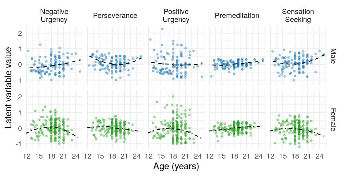
| UPPS-P factor | Sample | \(\text{Age}\) | \(\text{Age}\times\text{Gender}\) | \(\text{Age}^2\) | \(\text{Age}^2\times\text{Gender}\) |
|---|---|---|---|---|---|
| Neg Urgency | Adolescent | 0.01 [-0.14, 0.16] | -0.13 [-0.28, 0.01] | -0.07 [-0.21, 0.07] | -0.17 [-0.37, 0.02] |
| College | 0.01 [-0.11, 0.13] | -0.10 [-0.21, 0.01] | -0.07 [-0.20, 0.06] | -0.14 [-0.29, 0.02] | |
| Perseverance | Adolescent | -0.07 [-0.22, 0.08] | 0.04 [-0.10, 0.18] | 0.08 [-0.05, 0.21] | -0.21 [-0.37, -0.04] |
| College | -0.06 [-0.19, 0.07] | 0.03 [-0.08, 0.14] | 0.08 [-0.05, 0.20] | -0.17 [-0.30, -0.03] | |
| Pos Urgency | Adolescent | -0.03 [-0.17, 0.10] | -0.01 [-0.16, 0.13] | -0.05 [-0.18, 0.09] | -0.11 [-0.30, 0.08] |
| College | -0.03 [-0.14, 0.09] | -0.01 [-0.12, 0.10] | -0.04 [-0.17, 0.09] | -0.09 [-0.24, 0.07] | |
| Premeditation | Adolescent | 0.12 [-0.05, 0.28] | 0.04 [-0.13, 0.20] | 0.02 [-0.14, 0.18] | -0.07 [-0.28, 0.14] |
| College | 0.10 [-0.04, 0.23] | 0.03 [-0.10, 0.15] | 0.02 [-0.13, 0.17] | -0.05 [-0.22, 0.11] | |
| Sensation Seeking | Adolescent | 0.00 [-0.14, 0.14] | -0.11 [-0.27, 0.05] | 0.02 [-0.11, 0.14] | -0.19 [-0.37, -0.01] |
| College | 0.00 [-0.11, 0.11] | -0.08 [-0.19, 0.03] | 0.02 [-0.10, 0.13] | -0.15 [-0.28, -0.01] |
UPPS-P PDS
#>                                          df         AIC
#> uppsp_cfa_metric_pdssem_sample          355 38231.75325
#> uppsp_cfa_metric_pdssem_reginvar_sample 330 38215.01703
#> difference                              -25   -16.73621
#>                                             df        AIC
#> uppsp_cfa_metric_pdssemlin_reginvar_sample 320 38625.3327
#> uppsp_cfa_metric_pdssem_reginvar_sample    330 38215.0170
#> difference                                  10  -410.3157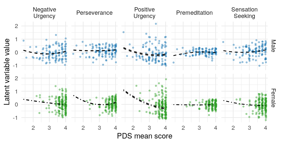
| UPPS-P factor | Sample | \(\text{PDS}\) | \(\text{PDS}\times\text{Gender}\) | \(\text{PDS}^2\) | \(\text{PDS}^2\times\text{Gender}\) |
|---|---|---|---|---|---|
| Neg Urgency | Adolescent | -0.06 [-0.31, 0.19] | -0.10 [-0.32, 0.12] | 0.07 [-0.13, 0.27] | -0.07 [-0.34, 0.19] |
| College | -0.04 [-0.18, 0.11] | -0.14 [-0.43, 0.16] | 0.05 [-0.10, 0.20] | -0.08 [-0.38, 0.22] | |
| Perseverance | Adolescent | -0.04 [-0.29, 0.22] | -0.07 [-0.29, 0.16] | 0.16 [-0.05, 0.36] | 0.16 [-0.12, 0.43] |
| College | -0.02 [-0.17, 0.13] | -0.09 [-0.39, 0.21] | 0.12 [-0.04, 0.27] | 0.17 [-0.13, 0.47] | |
| Pos Urgency | Adolescent | -0.26 [-0.49, -0.02] | -0.14 [-0.35, 0.07] | 0.10 [-0.10, 0.29] | 0.01 [-0.25, 0.26] |
| College | -0.15 [-0.29, -0.01] | -0.19 [-0.48, 0.10] | 0.07 [-0.07, 0.22] | 0.01 [-0.28, 0.30] | |
| Premeditation | Adolescent | 0.05 [-0.20, 0.30] | -0.04 [-0.26, 0.18] | -0.07 [-0.27, 0.13] | 0.12 [-0.15, 0.38] |
| College | 0.03 [-0.12, 0.17] | -0.06 [-0.36, 0.24] | -0.05 [-0.20, 0.10] | 0.13 [-0.17, 0.43] | |
| Sensation Seeking | Adolescent | -0.03 [-0.28, 0.23] | -0.11 [-0.34, 0.11] | 0.07 [-0.13, 0.28] | -0.02 [-0.29, 0.25] |
| College | -0.01 [-0.16, 0.13] | -0.15 [-0.45, 0.15] | 0.05 [-0.10, 0.20] | -0.02 [-0.32, 0.27] |
All latent var correlations
College sample
#>                              df      AIC
#> all_scales_college          679 54620.65
#> all_scales_college_cor      588 54564.95
#> all_scales_college_cor_load 583 54568.07
#>                                        df      AIC
#> all_scales_college_partnered          679 54533.51
#> all_scales_college_partnered_cor      588 54487.67
#> all_scales_college_partnered_cor_load 583 54486.70| rhs | 01. | 02. | 03. | 04. | 05. | 06. | 07. | 08. | 09. | 10. | 11. | 12. | 13. |
|---|---|---|---|---|---|---|---|---|---|---|---|---|---|
| 1. fsmi_mate | [-.09, .23] | [-.14, .15] | [-.17, .13] | [ .14, .43] | [-.25, .05] | [-.32,-.02] | [-.00, .30] | [ .14, .42] | [-.02, .27] | [ .08, .37] | [ .07, .38] | [ .06, .38] | |
| 2. fsmi_stat | .07 | [ .35, .63] | [ .62, .83] | [ .01, .35] | [ .12, .45] | [ .26, .57] | [ .14, .48] | [-.03, .31] | [ .53, .77] | [-.27, .07] | [ .27, .59] | [ .35, .66] | |
| 3. dominance_score | .01 | .49 | [ .07, .37] | [ .36, .62] | [-.31, .01] | [-.11, .22] | [ .20, .50] | [ .25, .52] | [ .02, .32] | [-.31, .01] | [-.01, .32] | [-.23, .12] | |
| 4. prestige_score | -.02 | .72 | .22 | [-.25, .07] | [ .23, .52] | [ .45, .69] | [ .09, .40] | [-.26, .05] | [ .36, .61] | [-.32,-.01] | [ .26, .56] | [ .26, .56] | |
| 5. neg_urgency | .29 | .18 | .49 | -.09 | [-.52,-.25] | [-.49,-.20] | [ .08, .39] | [ .70, .84] | [-.09, .22] | [ .04, .36] | [ .02, .35] | [-.08, .26] | |
| 6. premeditation | -.10 | .28 | -.15 | .38 | -.39 | [ .38, .64] | [-.38,-.08] | [-.53,-.26] | [ .00, .32] | [-.16, .17] | [-.20, .15] | [-.21, .14] | |
| 7. perseverance | -.17 | .41 | .05 | .57 | -.35 | .51 | [ .07, .38] | [-.43,-.14] | [ .14, .44] | [-.48,-.18] | [ .03, .37] | [-.00, .34] | |
| 8. sensation_seeking | .15 | .31 | .35 | .24 | .24 | -.23 | .23 | [ .12, .41] | [-.05, .28] | [-.26, .07] | [ .15, .48] | [ .08, .43] | |
| 9. pos_urgency | .28 | .14 | .39 | -.11 | .77 | -.40 | -.29 | .27 | [-.23, .08] | [ .02, .33] | [-.19, .15] | [-.29, .05] | |
| 10. k_srq_admiration | .12 | .65 | .17 | .49 | .06 | .16 | .29 | .12 | -.07 | [ .01, .31] | [ .59, .80] | [ .70, .88] | |
| 11. k_srq_passivity | .22 | -.10 | -.15 | -.17 | .20 | .00 | -.33 | -.10 | .18 | .16 | [-.06, .28] | [ .06, .40] | |
| 12. k_srq_sexual_relationships | .22 | .43 | .15 | .41 | .19 | -.03 | .20 | .32 | -.02 | .70 | .11 | [ .72, .94] | |
| 13. k_srq_sociability | .22 | .50 | -.06 | .41 | .09 | -.03 | .17 | .25 | -.12 | .79 | .23 | .83 |
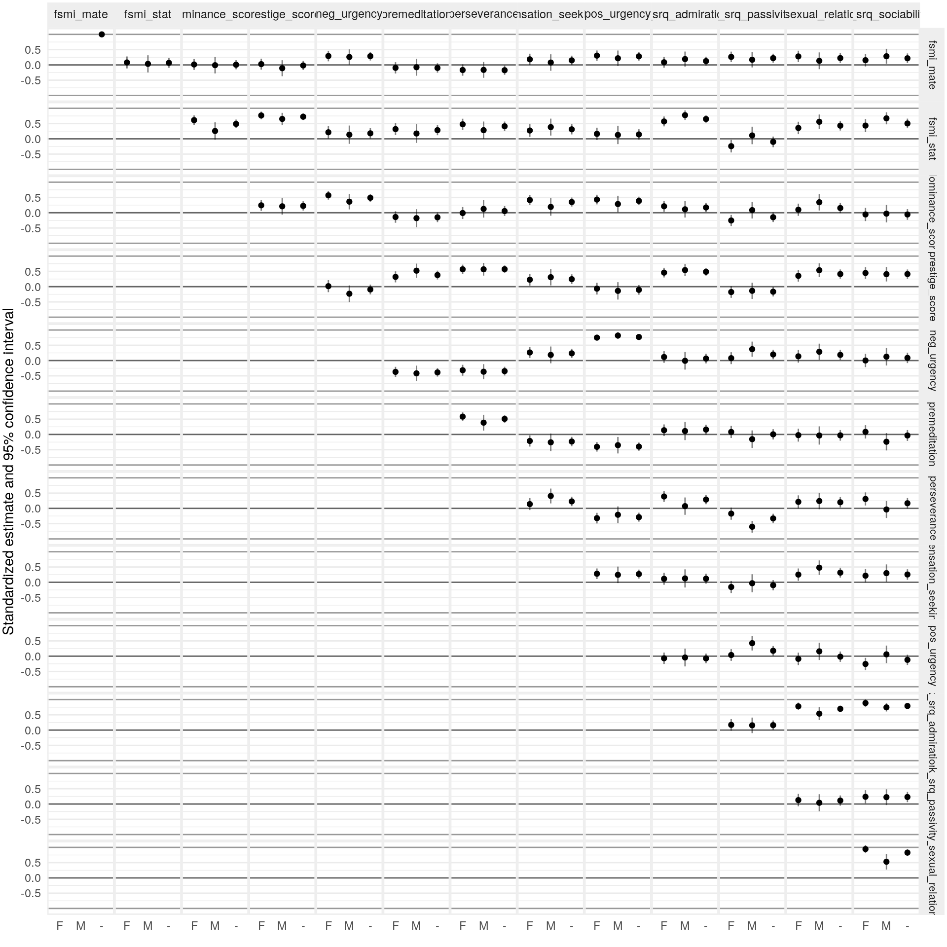
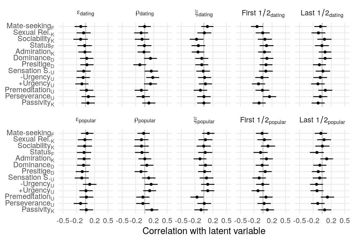
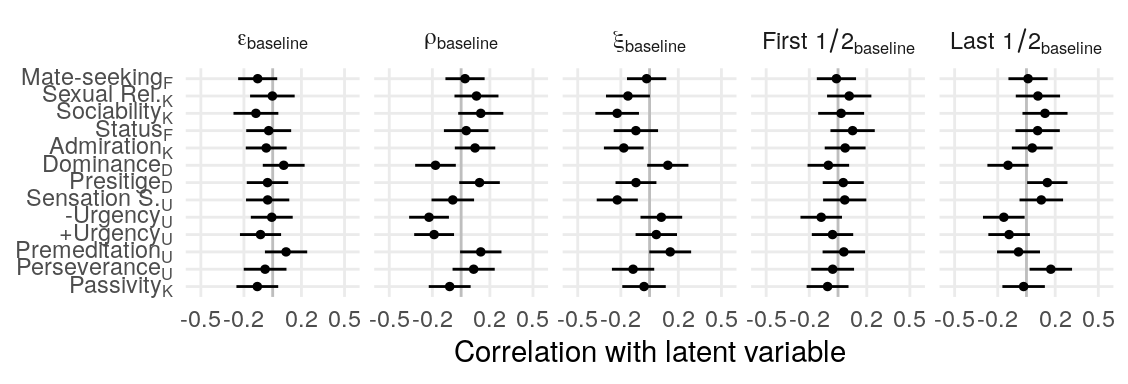
College and adolescent samples
#>                           df      AIC
#> all_scales_adol          831 51473.43
#> all_scales_adol_cor      696 51403.16
#> all_scales_adol_cor_load 684 51421.53
#> Chi-Squared Difference Test
#>
#>                             Df   AIC   BIC Chisq Chisq diff Df diff Pr(>Chisq)
#> all_scales_adol           9969 51473 54625 54270
#> all_scales_adol_cor      10104 51403 54043 54470    199.730     135   0.000249
#> all_scales_adol_cor_load 10116 51422 54016 54512     42.373      12  2.882e-05
#>
#> all_scales_adol
#> all_scales_adol_cor      ***
#> all_scales_adol_cor_load ***
#> ---
#> Signif. codes: 0 '***' 0.001 '**' 0.01 '*' 0.05 '.' 0.1 ' ' 1| rhs | 01. | 02. | 03. | 04. | 05. | 06. | 07. | 08. | 09. |
|---|---|---|---|---|---|---|---|---|---|
| 1. neg_urgency | [-.55,-.34] | [-.50,-.27] | [ .23, .47] | [ .71, .83] | [ .00, .27] | [-.05, .22] | [ .14, .39] | [-.02, .28] | |
| 2. premeditation | -.45 | [ .38, .59] | [-.43,-.19] | [-.54,-.33] | [-.04, .23] | [-.14, .13] | [-.22, .05] | [-.20, .11] | |
| 3. perseverance | -.38 | .49 | [-.02, .24] | [-.43,-.20] | [ .16, .41] | [-.39,-.13] | [-.03, .25] | [ .04, .34] | |
| 4. sensation_seeking | .35 | -.31 | .11 | [ .25, .47] | [ .09, .35] | [-.26, .02] | [ .27, .51] | [ .15, .44] | |
| 5. pos_urgency | .77 | -.43 | -.32 | .36 | [-.11, .15] | [-.01, .25] | [-.01, .26] | [-.18, .12] | |
| 6. k_srq_admiration | .14 | .09 | .29 | .22 | .02 | [-.07, .20] | [ .60, .77] | [ .64, .86] | |
| 7. k_srq_passivity | .08 | -.00 | -.26 | -.12 | .12 | .06 | [-.01, .26] | [ .05, .35] | |
| 8. k_srq_sexual_relationships | .27 | -.08 | .11 | .39 | .13 | .69 | .13 | [ .75, .94] | |
| 9. k_srq_sociability | .13 | -.04 | .19 | .30 | -.03 | .75 | .20 | .84 |
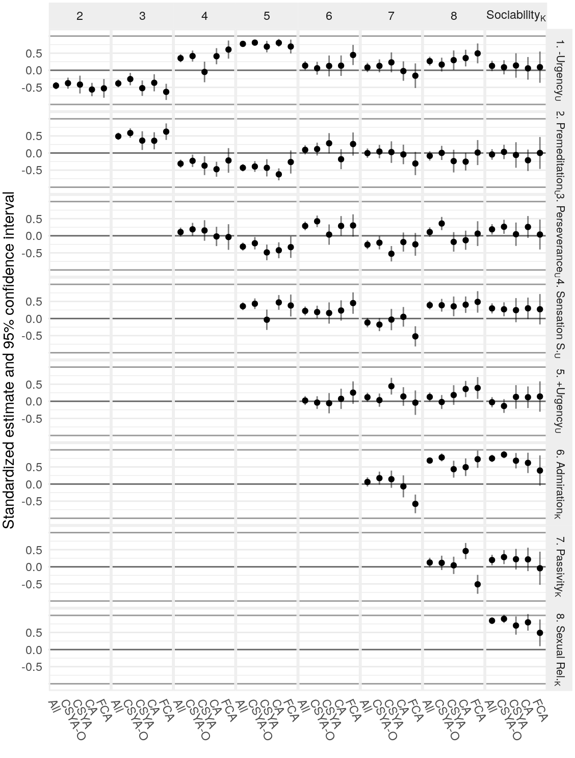
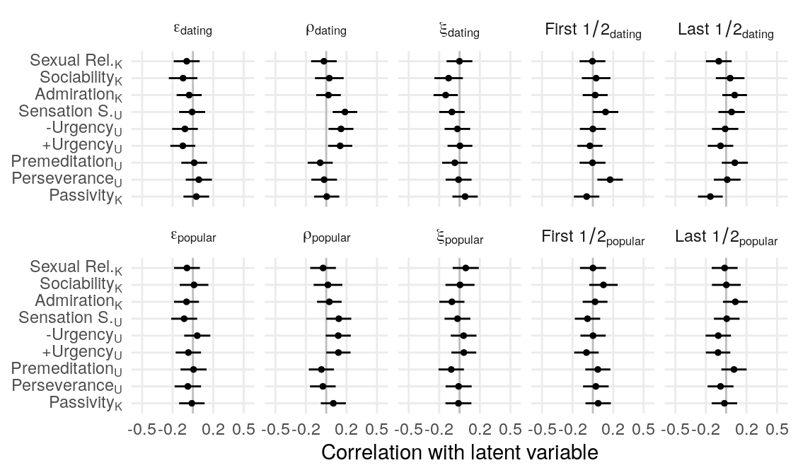
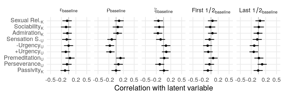
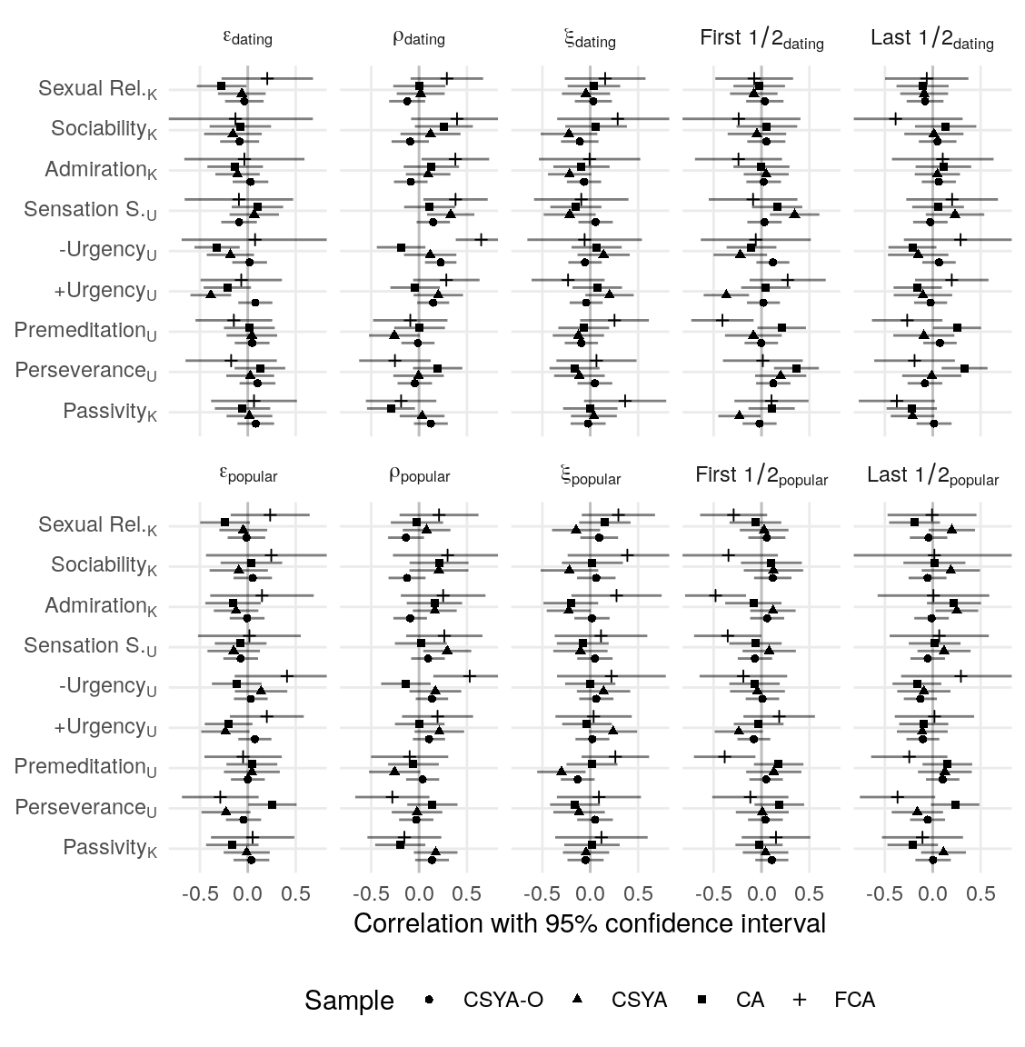
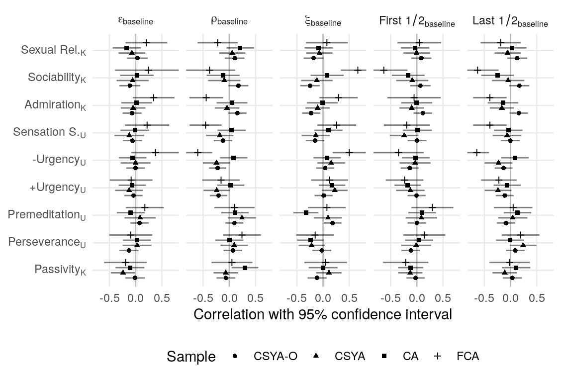
Associations with motive-relevant behavior
The number of partners and frequency of sex is expected to be different between those who are in or not in long-term relationships.
#>
#>              TDS1 TDS2 yads yads_online <NA>
#>   0             2   48   17          35    0
#>   1-9           1    7   33          28    0
#>   10-19         0    2    9          20    0
#>   20-39         1    4    8          23    0
#>   40 or more    1    0    6          27    0
#>   <NA>         34    4   11          12    1
#>
#>             TDS1 TDS2 yads yads_online <NA>
#>   0            2   48   17          35    0
#>   1            3   10   29          54    0
#>   2            0    4   17          19    0
#>   3 or more    1    3   18          29    0
#>   <NA>        33    0    3           8    1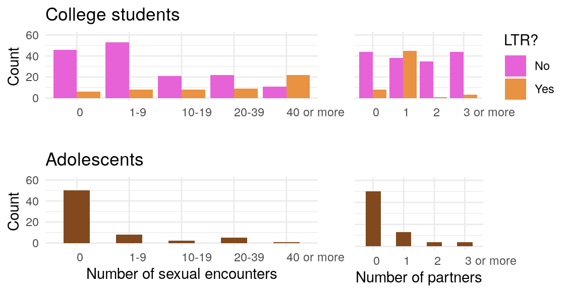
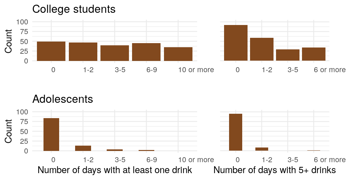
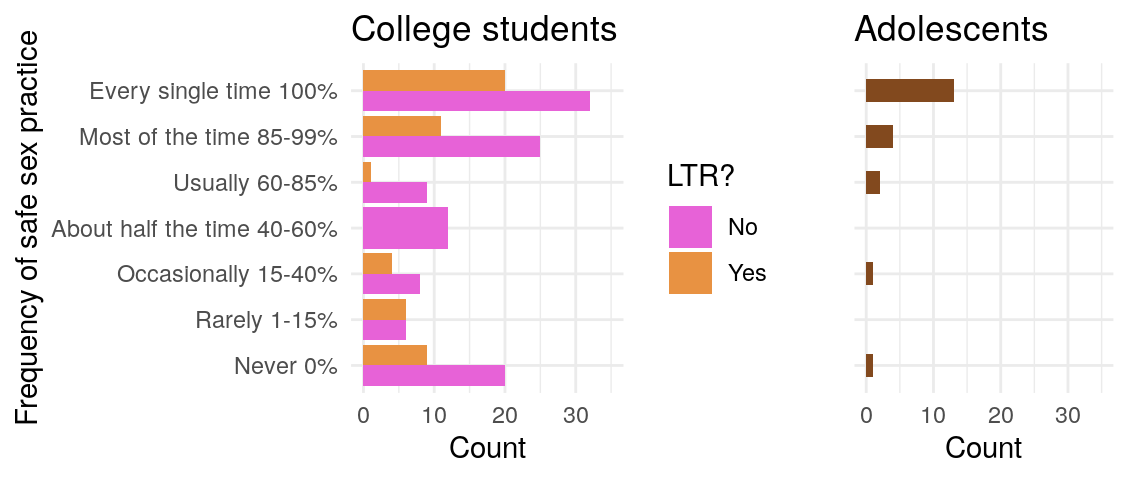
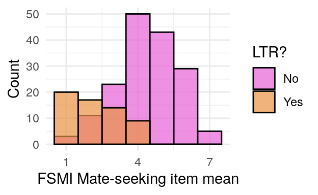
Number of partners
FSMI mate seeking
#> Scaled Chi Square Difference Test (method = "satorra.2000")
#>
#>                            Df AIC BIC  Chisq Chisq diff Df diff Pr(>Chisq)
#> fsmi_num_partners_sem      76         52.488
#> fsmi_num_partners_null_sem 77         66.939     4.7062       1    0.03005 *
#> ---
#> Signif. codes:  0 '***' 0.001 '**' 0.01 '*' 0.05 '.' 0.1 ' ' 1
#> Scaled Chi Square Difference Test (method = "satorra.2000")
#>
#>                                Df AIC BIC  Chisq Chisq diff Df diff Pr(>Chisq)
#> fsmi_num_partners_all_sem      76         68.846
#> fsmi_num_partners_null_all_sem 77         94.038     7.1694       1   0.007416
#>
#> fsmi_num_partners_all_sem
#> fsmi_num_partners_null_all_sem **
#> ---
#> Signif. codes:  0 '***' 0.001 '**' 0.01 '*' 0.05 '.' 0.1 ' ' 1
#> Scaled Chi Square Difference Test (method = "satorra.2000")
#>
#>                                 Df AIC BIC  Chisq Chisq diff Df diff Pr(>Chisq)
#> uppsp_fsmi_partners_sem        980         1210.6
#> uppsp_fsmi_partners_noupps_sem 983         1265.6     16.454   2.594  0.0005754
#> uppsp_fsmi_partners_null_sem   984         1387.8     19.020   1.000  1.294e-05
#>
#> uppsp_fsmi_partners_sem
#> uppsp_fsmi_partners_noupps_sem ***
#> uppsp_fsmi_partners_null_sem   ***
#> ---
#> Signif. codes:  0 '***' 0.001 '**' 0.01 '*' 0.05 '.' 0.1 ' ' 1
#> Scaled Chi Square Difference Test (method = "satorra.2000")
#>
#>                                 Df AIC BIC  Chisq Chisq diff Df diff Pr(>Chisq)
#> uppsp_fsmi_partners_sem        980         1210.6
#> uppsp_fsmi_partners_nofsmi_sem 981         1213.8     1.2595  1.0000     0.2617
#> uppsp_fsmi_partners_null_sem   984         1387.8    19.4231  1.8436  4.787e-05
#>
#> uppsp_fsmi_partners_sem
#> uppsp_fsmi_partners_nofsmi_sem
#> uppsp_fsmi_partners_null_sem   ***
#> ---
#> Signif. codes:  0 '***' 0.001 '**' 0.01 '*' 0.05 '.' 0.1 ' ' 1
#> Scaled Chi Square Difference Test (method = "satorra.2000")
#>
#>                                 Df AIC BIC  Chisq Chisq diff Df diff Pr(>Chisq)
#> uppsp_fsmi_partners_sem        980         1210.6
#> uppsp_fsmi_partners_nopurg_sem 981         1212.0     1.1041  1.0000     0.2934
#> uppsp_fsmi_partners_null_sem   984         1387.8    21.7578  2.1107  2.226e-05
#>
#> uppsp_fsmi_partners_sem
#> uppsp_fsmi_partners_nopurg_sem
#> uppsp_fsmi_partners_null_sem   ***
#> ---
#> Signif. codes:  0 '***' 0.001 '**' 0.01 '*' 0.05 '.' 0.1 ' ' 1
#> Scaled Chi Square Difference Test (method = "satorra.2000")
#>
#>                                 Df AIC BIC  Chisq Chisq diff Df diff Pr(>Chisq)
#> uppsp_fsmi_partners_sem        980         1210.6
#> uppsp_fsmi_partners_nonurg_sem 981         1210.8     0.2016  1.0000     0.6534
#> uppsp_fsmi_partners_null_sem   984         1387.8    21.8771  2.1188  2.123e-05
#>
#> uppsp_fsmi_partners_sem
#> uppsp_fsmi_partners_nonurg_sem
#> uppsp_fsmi_partners_null_sem   ***
#> ---
#> Signif. codes:  0 '***' 0.001 '**' 0.01 '*' 0.05 '.' 0.1 ' ' 1
#> Scaled Chi Square Difference Test (method = "satorra.2000")
#>
#>                               Df AIC BIC  Chisq Chisq diff Df diff Pr(>Chisq)
#> uppsp_fsmi_partners_sem      980         1210.6
#> uppsp_fsmi_partners_noss_sem 981         1212.9     0.7988  1.0000     0.3714
#> uppsp_fsmi_partners_null_sem 984         1387.8    20.3030  1.7431  2.621e-05
#>
#> uppsp_fsmi_partners_sem
#> uppsp_fsmi_partners_noss_sem
#> uppsp_fsmi_partners_null_sem ***
#> ---
#> Signif. codes:  0 '***' 0.001 '**' 0.01 '*' 0.05 '.' 0.1 ' ' 1
#>         est     pvalue
#> 1 0.1721959 0.02456491
#>        est      pvalue
#> 1 0.143696 0.006428484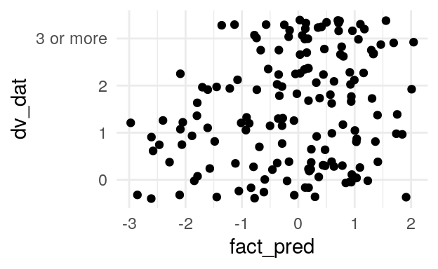
| lhs | op | rhs | est.std | se | z | pvalue | ci.lower | ci.upper |
|---|---|---|---|---|---|---|---|---|
| ordered_num_partner | ~ | fsmi_mate | 0.20 | 0.09 | 2.29 | 0.02 | 0.03 | 0.37 |
| ordered_num_partner | ~ | gender_c | -0.23 | 0.08 | -2.91 | 0.00 | -0.39 | -0.08 |
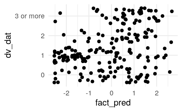
| lhs | op | rhs | est.std | se | z | pvalue | ci.lower | ci.upper |
|---|---|---|---|---|---|---|---|---|
| ordered_num_partner | ~ | fsmi_mate | 0.21 | 0.07 | 2.84 | 0 | 0.06 | 0.35 |
| ordered_num_partner | ~ | gender_c | -0.22 | 0.07 | -3.14 | 0 | -0.35 | -0.08 |
| lhs | op | rhs | est.std | se | z | pvalue | ci.lower | ci.upper |
|---|---|---|---|---|---|---|---|---|
| ordered_num_partner | ~ | neg_urgency | 0.10 | 0.21 | 0.45 | 0.65 | -0.32 | 0.51 |
| ordered_num_partner | ~ | sensation_seeking | 0.11 | 0.11 | 1.00 | 0.32 | -0.11 | 0.33 |
| ordered_num_partner | ~ | pos_urgency | 0.25 | 0.20 | 1.28 | 0.20 | -0.13 | 0.64 |
| ordered_num_partner | ~ | fsmi_mate | 0.00 | 0.00 | 0.00 | 0.00 | ||
| ordered_num_partner | ~ | gender_c | -0.22 | 0.09 | -2.45 | 0.01 | -0.39 | -0.04 |
| lhs | op | rhs | est.std | se | z | pvalue | ci.lower | ci.upper |
|---|---|---|---|---|---|---|---|---|
| ordered_num_partner | ~ | neg_urgency | 0.09 | 0.21 | 0.45 | 0.65 | -0.31 | 0.50 |
| ordered_num_partner | ~ | sensation_seeking | 0.10 | 0.11 | 0.89 | 0.37 | -0.12 | 0.31 |
| ordered_num_partner | ~ | pos_urgency | 0.21 | 0.20 | 1.06 | 0.29 | -0.18 | 0.61 |
| ordered_num_partner | ~ | fsmi_mate | 0.12 | 0.11 | 1.18 | 0.24 | -0.08 | 0.33 |
| ordered_num_partner | ~ | gender_c | -0.22 | 0.09 | -2.45 | 0.01 | -0.39 | -0.04 |
| lhs | op | rhs | est.std | se | z | pvalue | ci.lower | ci.upper |
|---|---|---|---|---|---|---|---|---|
| ordered_num_partner | ~ | neg_urgency | 0.15 | 0.19 | 0.79 | 0.43 | -0.23 | 0.53 |
| ordered_num_partner | ~ | sensation_seeking | 0.08 | 0.09 | 0.84 | 0.40 | -0.10 | 0.26 |
| ordered_num_partner | ~ | pos_urgency | 0.08 | 0.19 | 0.46 | 0.65 | -0.28 | 0.45 |
| ordered_num_partner | ~ | fsmi_mate | 0.14 | 0.09 | 1.62 | 0.11 | -0.03 | 0.31 |
| ordered_num_partner | ~ | gender_c | -0.22 | 0.08 | -2.81 | 0.01 | -0.37 | -0.07 |
The basic takeaway from the above is that a lot of these are associated but remove any one of them and model fit doesn’t drop much. Remove a couple (both urgency scales, or all upps-p scales) and there’s a big model fit drop. Include only one, and then remove it, and there’s a big model fit drop. For now, I’m going to stick with just describing the relations with the motive scales. When looking at the size of standardized coefficients, positive urgency is the largest, and is not greatly diminished by the addition of the FSMI Mate-seeking scale.
K-SRQ sexual relationship
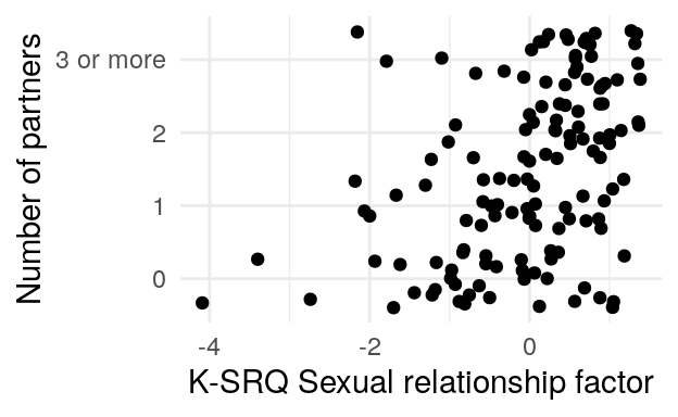
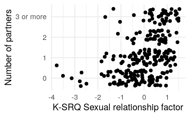
#> Scaled Chi Square Difference Test (method = "satorra.2000")
#>
#>                                Df AIC BIC   Chisq Chisq diff Df diff Pr(>Chisq)
#> ksrq_noadmrtn_num_partners_sem 84          58.306
#> ksrq_num_partners_null_sem     85         116.360     11.239       1  0.0008009
#>
#> ksrq_noadmrtn_num_partners_sem
#> ksrq_num_partners_null_sem     ***
#> ---
#> Signif. codes:  0 '***' 0.001 '**' 0.01 '*' 0.05 '.' 0.1 ' ' 1
#> Scaled Chi Square Difference Test (method = "satorra.2000")
#>
#>                                    Df AIC BIC  Chisq Chisq diff Df diff
#> ksrq_noadmrtn_num_partners_all_sem 97         161.95
#> ksrq_num_partners_null_all_sem     98         268.17     24.128       1
#>                                    Pr(>Chisq)
#> ksrq_noadmrtn_num_partners_all_sem
#> ksrq_num_partners_null_all_sem      9.015e-07 ***
#> ---
#> Signif. codes:  0 '***' 0.001 '**' 0.01 '*' 0.05 '.' 0.1 ' ' 1
#> Scaled Chi Square Difference Test (method = "satorra.2000")
#>
#>                                Df AIC BIC  Chisq Chisq diff Df diff Pr(>Chisq)
#> ksrq_num_partners_sem          83         56.291
#> ksrq_noadmrtn_num_partners_sem 84         58.306      2.126       1     0.1448
#> Scaled Chi Square Difference Test (method = "satorra.2000")
#>
#>                                    Df AIC BIC  Chisq Chisq diff Df diff
#> uppsp_ksrq_num_partners_sem      1301         1510.5
#> uppsp_ksrq_nosr_num_partners_sem 1302         1527.5     7.6722       1
#>                                  Pr(>Chisq)
#> uppsp_ksrq_num_partners_sem
#> uppsp_ksrq_nosr_num_partners_sem   0.005608 **
#> ---
#> Signif. codes:  0 '***' 0.001 '**' 0.01 '*' 0.05 '.' 0.1 ' ' 1
#> Scaled Chi Square Difference Test (method = "satorra.2000")
#>
#>                                         Df AIC BIC  Chisq Chisq diff Df diff
#> uppsp_ksrq_num_partners_all__sem      1352         2114.7
#> uppsp_ksrq_nosr_num_partners_all__sem 1353         2154.3     22.914       1
#>                                       Pr(>Chisq)
#> uppsp_ksrq_num_partners_all__sem
#> uppsp_ksrq_nosr_num_partners_all__sem  1.694e-06 ***
#> ---
#> Signif. codes: 0 '***' 0.001 '**' 0.01 '*' 0.05 '.' 0.1 ' ' 1| lhs | op | rhs | est | se | z | pvalue | ci.lower | ci.upper | std.lv | std.all | std.nox |
|---|---|---|---|---|---|---|---|---|---|---|---|
| ordered_num_partner | ~ | k_srq_sexual_relationships | 0.52 | 0.13 | 4.04 | 0.00 | 0.27 | 0.77 | 0.56 | 0.55 | 0.55 |
| ordered_num_partner | ~ | k_srq_admiration | -0.21 | 0.14 | -1.51 | 0.13 | -0.48 | 0.06 | -0.21 | -0.21 | -0.21 |
| ordered_num_partner | ~ | gender_c | -0.39 | 0.20 | -2.00 | 0.05 | -0.77 | -0.01 | -0.39 | -0.18 | -0.38 |
| lhs | op | rhs | est | se | z | pvalue | ci.lower | ci.upper | std.lv | std.all | std.nox |
|---|---|---|---|---|---|---|---|---|---|---|---|
| ordered_num_partner | ~ | k_srq_sexual_relationships | 0.33 | 0.09 | 3.49 | 0.00 | 0.14 | 0.51 | 0.36 | 0.35 | 0.35 |
| ordered_num_partner | ~ | k_srq_admiration | 0.00 | 0.00 | 0.00 | 0.00 | 0.00 | 0.00 | 0.00 | ||
| ordered_num_partner | ~ | gender_c | -0.39 | 0.20 | -2.00 | 0.05 | -0.77 | -0.01 | -0.39 | -0.18 | -0.38 |
| lhs | op | rhs | est | se | z | pvalue | ci.lower | ci.upper | std.lv | std.all | std.nox |
|---|---|---|---|---|---|---|---|---|---|---|---|
| ordered_num_partner | ~ | k_srq_sexual_relationships | 0.77 | 0.12 | 6.46 | 0.00 | 0.54 | 1.00 | 0.78 | 0.71 | 0.71 |
| ordered_num_partner | ~ | k_srq_admiration | -0.47 | 0.11 | -4.13 | 0.00 | -0.70 | -0.25 | -0.43 | -0.39 | -0.39 |
| ordered_num_partner | ~ | gender_c | -0.04 | 0.15 | -0.24 | 0.81 | -0.33 | 0.26 | -0.04 | -0.02 | -0.03 |
| ordered_num_partner | ~ | age_c | 0.22 | 0.04 | 6.12 | 0.00 | 0.15 | 0.28 | 0.22 | 0.43 | 0.19 |
| lhs | op | rhs | est | se | z | pvalue | ci.lower | ci.upper | std.lv | std.all | std.nox |
|---|---|---|---|---|---|---|---|---|---|---|---|
| ordered_num_partner | ~ | k_srq_sexual_relationships | 0.36 | 0.07 | 4.92 | 0.00 | 0.22 | 0.50 | 0.38 | 0.34 | 0.34 |
| ordered_num_partner | ~ | k_srq_admiration | 0.00 | 0.00 | 0.00 | 0.00 | 0.00 | 0.00 | 0.00 | ||
| ordered_num_partner | ~ | gender_c | -0.04 | 0.15 | -0.24 | 0.81 | -0.33 | 0.26 | -0.04 | -0.02 | -0.03 |
| ordered_num_partner | ~ | age_c | 0.22 | 0.04 | 6.12 | 0.00 | 0.15 | 0.28 | 0.22 | 0.43 | 0.19 |
| lhs | op | rhs | est | se | z | pvalue | ci.lower | ci.upper | std.lv | std.all | std.nox |
|---|---|---|---|---|---|---|---|---|---|---|---|
| ordered_num_partner | ~ | neg_urgency | -0.28 | 0.53 | -0.52 | 0.60 | -1.31 | 0.76 | -0.11 | -0.11 | -0.11 |
| ordered_num_partner | ~ | sensation_seeking | -0.22 | 0.36 | -0.62 | 0.53 | -0.93 | 0.48 | -0.09 | -0.09 | -0.09 |
| ordered_num_partner | ~ | pos_urgency | 0.70 | 0.38 | 1.85 | 0.06 | -0.04 | 1.44 | 0.39 | 0.38 | 0.38 |
| ordered_num_partner | ~ | k_srq_sexual_relationships | 0.34 | 0.13 | 2.61 | 0.01 | 0.08 | 0.60 | 0.41 | 0.40 | 0.40 |
| ordered_num_partner | ~ | gender_c | -0.38 | 0.21 | -1.82 | 0.07 | -0.79 | 0.03 | -0.38 | -0.17 | -0.38 |
| lhs | op | rhs | est | se | z | pvalue | ci.lower | ci.upper | std.lv | std.all | std.nox |
|---|---|---|---|---|---|---|---|---|---|---|---|
| ordered_num_partner | ~ | neg_urgency | 1.29 | 0.70 | 1.83 | 0.07 | -0.09 | 2.66 | 0.53 | 0.52 | 0.52 |
| ordered_num_partner | ~ | sensation_seeking | 0.41 | 0.33 | 1.26 | 0.21 | -0.23 | 1.06 | 0.16 | 0.16 | 0.16 |
| ordered_num_partner | ~ | pos_urgency | -0.34 | 0.44 | -0.76 | 0.45 | -1.20 | 0.53 | -0.19 | -0.18 | -0.18 |
| ordered_num_partner | ~ | k_srq_sexual_relationships | 0.00 | 0.00 | 0.00 | 0.00 | 0.00 | 0.00 | 0.00 | ||
| ordered_num_partner | ~ | gender_c | -0.38 | 0.21 | -1.82 | 0.07 | -0.79 | 0.03 | -0.38 | -0.17 | -0.38 |
| lhs | op | rhs | est | se | z | pvalue | ci.lower | ci.upper | std.lv | std.all | std.nox |
|---|---|---|---|---|---|---|---|---|---|---|---|
| ordered_num_partner | ~ | neg_urgency | -0.46 | 0.37 | -1.26 | 0.21 | -1.18 | 0.26 | -0.23 | -0.21 | -0.21 |
| ordered_num_partner | ~ | sensation_seeking | -0.02 | 0.21 | -0.11 | 0.91 | -0.44 | 0.39 | -0.01 | -0.01 | -0.01 |
| ordered_num_partner | ~ | pos_urgency | 0.83 | 0.28 | 2.93 | 0.00 | 0.27 | 1.38 | 0.53 | 0.48 | 0.48 |
| ordered_num_partner | ~ | k_srq_sexual_relationships | 0.39 | 0.09 | 4.39 | 0.00 | 0.22 | 0.57 | 0.43 | 0.39 | 0.39 |
| ordered_num_partner | ~ | gender_c | -0.07 | 0.16 | -0.42 | 0.67 | -0.38 | 0.25 | -0.07 | -0.03 | -0.06 |
| ordered_num_partner | ~ | age_c | 0.21 | 0.04 | 5.49 | 0.00 | 0.13 | 0.28 | 0.21 | 0.42 | 0.19 |
| lhs | op | rhs | est | se | z | pvalue | ci.lower | ci.upper | std.lv | std.all | std.nox |
|---|---|---|---|---|---|---|---|---|---|---|---|
| ordered_num_partner | ~ | neg_urgency | 2.62 | 0.86 | 3.05 | 0.00 | 0.94 | 4.30 | 1.24 | 1.13 | 1.13 |
| ordered_num_partner | ~ | sensation_seeking | 0.33 | 0.24 | 1.39 | 0.16 | -0.14 | 0.80 | 0.15 | 0.14 | 0.14 |
| ordered_num_partner | ~ | pos_urgency | -1.41 | 0.58 | -2.42 | 0.02 | -2.56 | -0.27 | -0.89 | -0.81 | -0.81 |
| ordered_num_partner | ~ | k_srq_sexual_relationships | 0.00 | 0.00 | 0.00 | 0.00 | 0.00 | 0.00 | 0.00 | ||
| ordered_num_partner | ~ | gender_c | -0.07 | 0.16 | -0.42 | 0.67 | -0.38 | 0.25 | -0.07 | -0.03 | -0.06 |
| ordered_num_partner | ~ | age_c | 0.21 | 0.04 | 5.49 | 0.00 | 0.13 | 0.28 | 0.21 | 0.42 | 0.19 |
K-SRQ Sexual Relationships is associated with number of sexual partners in both the unpartnered college sample, and the combined adolescent and college sample. There are too few participants in the adolescent sample with one or more sexual partners so while some of the analyses do use data from all participants with responses on the SES, this primarily serves to integrate both partnered and upartnered college students. Notably, the standardized coefficient for the association between number of sexual partners and K-SRQ Sexual Relationships does not change much between either the full, or unpartnered college students subgroups. Sociability and Sexual Relationships are too highly correlated to be disentangled. Controlling for the other highly correlated K-SRQ scale, Admiration, yields a standardized effect of Sexual Relationships that has the same sign, but that has bigger magnitude. The coefficient for the Admiration scale is large and negative, which evokes extremely speculative narratives having to do with reputational concerns and promiscuity. The magnitude of the Sexual Relationships association (the standard deviation is close to one, so the standardized and unstandardized coefficients are very similar) is about the same size as the effect of reported gender. In other words, the expected difference in number of sexual partners a one point increase on K-SRQ Sexual Relationshi
SPLT parameters
#> Scaled Chi Square Difference Test (method = "satorra.2000")
#>
#>                            Df AIC BIC   Chisq Chisq diff Df diff Pr(>Chisq)
#> splt_num_partners_sem       9          3.9468
#> splt_num_partners_null_sem 10         19.1986     4.9983       1    0.02537 *
#> ---
#> Signif. codes:  0 '***' 0.001 '**' 0.01 '*' 0.05 '.' 0.1 ' ' 1
#> Scaled Chi Square Difference Test (method = "satorra.2000")
#>
#>                                Df AIC BIC  Chisq Chisq diff Df diff Pr(>Chisq)
#> splt_num_partners_all_sem      14         22.252
#> splt_num_partners_all_null_sem 15         32.547     3.6398       1    0.05641
#>
#> splt_num_partners_all_sem
#> splt_num_partners_all_null_sem .
#> ---
#> Signif. codes:  0 '***' 0.001 '**' 0.01 '*' 0.05 '.' 0.1 ' ' 1
#> Scaled Chi Square Difference Test (method = "satorra.2000")
#>
#>                            Df AIC BIC  Chisq Chisq diff Df diff Pr(>Chisq)
#> splt_num_partners_sem       9         5.5471
#> splt_num_partners_null_sem 10         6.2243    0.16057       1     0.6886
#> Scaled Chi Square Difference Test (method = "satorra.2000")
#>
#>                                Df AIC BIC  Chisq Chisq diff Df diff Pr(>Chisq)
#> splt_num_partners_all_sem      14         10.312
#> splt_num_partners_all_null_sem 15         14.200    0.94236       1     0.3317
#> Scaled Chi Square Difference Test (method = "satorra.2000")
#>
#>                            Df AIC BIC   Chisq Chisq diff Df diff Pr(>Chisq)
#> splt_num_partners_sem       9          9.1953
#> splt_num_partners_null_sem 10         10.4587    0.80258       1     0.3703
#> Scaled Chi Square Difference Test (method = "satorra.2000")
#>
#>                                Df AIC BIC   Chisq Chisq diff Df diff Pr(>Chisq)
#> splt_num_partners_all_sem      14          8.3193
#> splt_num_partners_all_null_sem 15         10.6411     1.5034       1     0.2202
#> Scaled Chi Square Difference Test (method = "satorra.2000")
#>
#>                            Df AIC BIC  Chisq Chisq diff Df diff Pr(>Chisq)
#> splt_num_partners_sem       9         2.2235
#> splt_num_partners_null_sem 10         2.5325    0.15418       1     0.6946
#> Scaled Chi Square Difference Test (method = "satorra.2000")
#>
#>                                Df AIC BIC  Chisq Chisq diff Df diff Pr(>Chisq)
#> splt_num_partners_all_sem      14         7.9255
#> splt_num_partners_all_null_sem 15         8.0706   0.065488       1      0.798
#> Scaled Chi Square Difference Test (method = "satorra.2000")
#>
#>                            Df AIC BIC  Chisq Chisq diff Df diff Pr(>Chisq)
#> splt_num_partners_sem       9          8.759
#> splt_num_partners_null_sem 10         13.489     2.5065       1     0.1134
#> Scaled Chi Square Difference Test (method = "satorra.2000")
#>
#>                                Df AIC BIC  Chisq Chisq diff Df diff Pr(>Chisq)
#> splt_num_partners_all_sem      14         24.501
#> splt_num_partners_all_null_sem 15         25.956    0.76758       1      0.381
#> Scaled Chi Square Difference Test (method = "satorra.2000")
#>
#>                            Df AIC BIC   Chisq Chisq diff Df diff Pr(>Chisq)
#> splt_num_partners_sem       9          6.8394
#> splt_num_partners_null_sem 10         10.1926     1.9798       1     0.1594
#> Scaled Chi Square Difference Test (method = "satorra.2000")
#>
#>                                Df AIC BIC   Chisq Chisq diff Df diff Pr(>Chisq)
#> splt_num_partners_all_sem      14          9.2835
#> splt_num_partners_all_null_sem 15         17.1682     4.9204       1    0.02654
#>
#> splt_num_partners_all_sem
#> splt_num_partners_all_null_sem *
#> ---
#> Signif. codes:  0 '***' 0.001 '**' 0.01 '*' 0.05 '.' 0.1 ' ' 1
#>
#>
#> Table: (\#tab:unnamed-chunk-50)$\epsilon$ predicting number of partners among unpartnered college students; N obs. = 159
#>
#> lhs                   op   rhs                       est     se       z   pvalue   ci.lower   ci.upper   std.lv   std.all   std.nox
#> --------------------  ---  ---------------------  ------  -----  ------  -------  ---------  ---------  -------  --------  --------
#> ordered_num_partner   ~    ep_prm_DtngLHngT_fac    -3.45   1.50   -2.30     0.02      -6.38      -0.52    -0.22     -0.21     -0.21
#> ordered_num_partner   ~    gender_c                -0.57   0.18   -3.15     0.00      -0.93      -0.22    -0.57     -0.26     -0.55
#>
#>
#> Table: (\#tab:unnamed-chunk-50)$\epsilon$ predicting number of partners among all adolescent and college participants with SES responses; N obs. = 276
#>
#> lhs                   op   rhs                       est     se       z   pvalue   ci.lower   ci.upper   std.lv   std.all   std.nox
#> --------------------  ---  ---------------------  ------  -----  ------  -------  ---------  ---------  -------  --------  --------
#> ordered_num_partner   ~    ep_prm_DtngLHngT_fac    -2.39   1.23   -1.94     0.05      -4.81       0.03    -0.14     -0.13     -0.13
#> ordered_num_partner   ~    gender_c                -0.16   0.14   -1.09     0.28      -0.44       0.12    -0.16     -0.07     -0.14
#> ordered_num_partner   ~    age_c                    0.20   0.03    5.78     0.00       0.13       0.27     0.20      0.40      0.18
#>
#>
#> Table: (\#tab:unnamed-chunk-50)$\rho$ predicting number of partners among unpartnered college students; N obs. = 159
#>
#> lhs                   op   rhs                        est     se       z   pvalue   ci.lower   ci.upper   std.lv   std.all   std.nox
#> --------------------  ---  ----------------------  ------  -----  ------  -------  ---------  ---------  -------  --------  --------
#> ordered_num_partner   ~    rho_prm_DtngLHngT_fac     0.05   0.13    0.40     0.69      -0.21       0.32     0.04      0.04      0.04
#> ordered_num_partner   ~    gender_c                 -0.57   0.18   -3.15     0.00      -0.93      -0.22    -0.57     -0.26     -0.55
#>
#>
#> Table: (\#tab:unnamed-chunk-50)$\rho$ predicting number of partners among all adolescent and college participants with SES responses; N obs. = 276
#>
#> lhs                   op   rhs                        est     se       z   pvalue   ci.lower   ci.upper   std.lv   std.all   std.nox
#> --------------------  ---  ----------------------  ------  -----  ------  -------  ---------  ---------  -------  --------  --------
#> ordered_num_partner   ~    rho_prm_DtngLHngT_fac     0.10   0.11    0.97     0.33      -0.11       0.32     0.07      0.06      0.06
#> ordered_num_partner   ~    gender_c                 -0.16   0.14   -1.09     0.28      -0.44       0.12    -0.16     -0.07     -0.14
#> ordered_num_partner   ~    age_c                     0.20   0.03    5.78     0.00       0.13       0.27     0.20      0.40      0.18
#>
#>
#> Table: (\#tab:unnamed-chunk-50)$\xi$ predicting number of partners among unpartnered college students; N obs. = 159
#>
#> lhs                   op   rhs                       est     se       z   pvalue   ci.lower   ci.upper   std.lv   std.all   std.nox
#> --------------------  ---  ---------------------  ------  -----  ------  -------  ---------  ---------  -------  --------  --------
#> ordered_num_partner   ~    xi_prm_DtngLHngT_fac     0.87   0.99    0.88     0.38      -1.07       2.82     0.07      0.07      0.07
#> ordered_num_partner   ~    gender_c                -0.57   0.18   -3.15     0.00      -0.93      -0.22    -0.57     -0.26     -0.55
#>
#>
#> Table: (\#tab:unnamed-chunk-50)$\xi$ predicting number of partners among all adolescent and college participants with SES responses; N obs. = 276
#>
#> lhs                   op   rhs                       est     se       z   pvalue   ci.lower   ci.upper   std.lv   std.all   std.nox
#> --------------------  ---  ---------------------  ------  -----  ------  -------  ---------  ---------  -------  --------  --------
#> ordered_num_partner   ~    xi_prm_DtngLHngT_fac     1.07   0.90    1.20     0.23      -0.69       2.83     0.08      0.07      0.07
#> ordered_num_partner   ~    gender_c                -0.16   0.14   -1.09     0.28      -0.44       0.12    -0.16     -0.07     -0.14
#> ordered_num_partner   ~    age_c                    0.20   0.03    5.78     0.00       0.13       0.27     0.20      0.40      0.18
#>
#>
#> Table: (\#tab:unnamed-chunk-50)$b$ predicting number of partners among unpartnered college students; N obs. = 159
#>
#> lhs                   op   rhs                  est     se       z   pvalue   ci.lower   ci.upper   std.lv   std.all   std.nox
#> --------------------  ---  ----------------  ------  -----  ------  -------  ---------  ---------  -------  --------  --------
#> ordered_num_partner   ~    b_DtngLHngT_fac     0.13   0.33    0.39     0.69      -0.52       0.78     0.03      0.03      0.03
#> ordered_num_partner   ~    gender_c           -0.57   0.18   -3.15     0.00      -0.93      -0.22    -0.57     -0.26     -0.55
#>
#>
#> Table: (\#tab:unnamed-chunk-50)$b$ predicting number of partners among all adolescent and college participants with SES responses; N obs. = 276
#>
#> lhs                   op   rhs                  est     se       z   pvalue   ci.lower   ci.upper   std.lv   std.all   std.nox
#> --------------------  ---  ----------------  ------  -----  ------  -------  ---------  ---------  -------  --------  --------
#> ordered_num_partner   ~    b_DtngLHngT_fac     0.06   0.22    0.26     0.80      -0.38       0.49     0.02      0.02      0.02
#> ordered_num_partner   ~    gender_c           -0.16   0.14   -1.09     0.28      -0.44       0.12    -0.16     -0.07     -0.14
#> ordered_num_partner   ~    age_c               0.20   0.03    5.78     0.00       0.13       0.27     0.20      0.40      0.18
#>
#>
#> Table: (\#tab:unnamed-chunk-50)First-half optimal responses predicting number of partners among unpartnered college students; N obs. = 159
#>
#> lhs                   op   rhs                               est     se       z   pvalue   ci.lower   ci.upper   std.lv   std.all   std.nox
#> --------------------  ---  -----------------------------  ------  -----  ------  -------  ---------  ---------  -------  --------  --------
#> ordered_num_partner   ~    bin_start_to_4_DtngLHngT_fac    -0.94   0.59   -1.60     0.11      -2.09       0.21    -0.14     -0.13     -0.13
#> ordered_num_partner   ~    gender_c                        -0.57   0.18   -3.15     0.00      -0.93      -0.22    -0.57     -0.26     -0.55
#>
#>
#> Table: (\#tab:unnamed-chunk-50)First-half optimal responses predicting number of partners among all adolescent and college participants with SES responses; N obs. = 276
#>
#> lhs                   op   rhs                               est     se       z   pvalue   ci.lower   ci.upper   std.lv   std.all   std.nox
#> --------------------  ---  -----------------------------  ------  -----  ------  -------  ---------  ---------  -------  --------  --------
#> ordered_num_partner   ~    bin_start_to_4_DtngLHngT_fac    -0.42   0.47   -0.88     0.38      -1.34       0.51    -0.06     -0.05     -0.05
#> ordered_num_partner   ~    gender_c                        -0.16   0.14   -1.09     0.28      -0.44       0.12    -0.16     -0.07     -0.14
#> ordered_num_partner   ~    age_c                            0.20   0.03    5.78     0.00       0.13       0.27     0.20      0.40      0.18
#>
#>
#> Table: (\#tab:unnamed-chunk-50)Last-half optimal responses predicting number of partners among unpartnered college students; N obs. = 159
#>
#> lhs                   op   rhs                             est     se       z   pvalue   ci.lower   ci.upper   std.lv   std.all   std.nox
#> --------------------  ---  ---------------------------  ------  -----  ------  -------  ---------  ---------  -------  --------  --------
#> ordered_num_partner   ~    bin_5_to_end_DtngLHngT_fac    -0.77   0.55   -1.39     0.16      -1.85       0.31    -0.12     -0.11     -0.11
#> ordered_num_partner   ~    gender_c                      -0.57   0.18   -3.15     0.00      -0.93      -0.22    -0.57     -0.26     -0.55
#>
#>
#> Table: (\#tab:unnamed-chunk-50)Last-half optimal responses predicting number of partners among all adolescent and college participants with SES responses; N obs. = 276
#>
#> lhs                   op   rhs                             est     se       z   pvalue   ci.lower   ci.upper   std.lv   std.all   std.nox
#> --------------------  ---  ---------------------------  ------  -----  ------  -------  ---------  ---------  -------  --------  --------
#> ordered_num_partner   ~    bin_5_to_end_DtngLHngT_fac    -1.01   0.46   -2.18     0.03      -1.91      -0.10    -0.15     -0.13     -0.13
#> ordered_num_partner   ~    gender_c                      -0.16   0.14   -1.09     0.28      -0.44       0.12    -0.16     -0.07     -0.14
#> ordered_num_partner   ~    age_c                          0.20   0.03    5.78     0.00       0.13       0.27     0.20      0.40      0.18
No \(\chi^2\) tests satisfy the \(\alpha = .005\) cutoff. The biggest association is with the \(\epsilon\) contrast variable, but it has the wrong sign, with higher learning rates being associated with fewer numbers of sexual partners.
Number of sexual encounters
FSMI mate seeking
#> Scaled Chi Square Difference Test (method = "satorra.2000")
#>
#>                        Df AIC BIC  Chisq Chisq diff Df diff Pr(>Chisq)
#> fsmi_sex_freq_sem      76         57.092
#> fsmi_sex_freq_null_sem 77         62.718     1.7438       1     0.1867
#> Scaled Chi Square Difference Test (method = "satorra.2000")
#>
#>                              Df AIC BIC  Chisq Chisq diff Df diff Pr(>Chisq)
#> uppsp_fsmi_sfreq_sem        980         1220.0
#> uppsp_fsmi_sfreq_noupps_sem 983         1286.9    13.1532  2.2516   0.001907 **
#> uppsp_fsmi_sfreq_null_sem   984         1288.9     0.2936  1.0000   0.587904
#> ---
#> Signif. codes:  0 '***' 0.001 '**' 0.01 '*' 0.05 '.' 0.1 ' ' 1
#> Scaled Chi Square Difference Test (method = "satorra.2000")
#>
#>                              Df AIC BIC  Chisq Chisq diff Df diff Pr(>Chisq)
#> uppsp_fsmi_sfreq_sem        980         1220.0
#> uppsp_fsmi_sfreq_nofsmi_sem 981         1235.1     5.6190  1.0000    0.01777 *
#> uppsp_fsmi_sfreq_null_sem   984         1288.9     6.2027  1.8379    0.03816 *
#> ---
#> Signif. codes:  0 '***' 0.001 '**' 0.01 '*' 0.05 '.' 0.1 ' ' 1
#> Scaled Chi Square Difference Test (method = "satorra.2000")
#>
#>                              Df AIC BIC  Chisq Chisq diff Df diff Pr(>Chisq)
#> uppsp_fsmi_sfreq_sem        980         1220.0
#> uppsp_fsmi_sfreq_nopurg_sem 981         1220.0     0.0061  1.0000    0.93785
#> uppsp_fsmi_sfreq_null_sem   984         1288.9     8.1421  2.0259    0.01755 *
#> ---
#> Signif. codes:  0 '***' 0.001 '**' 0.01 '*' 0.05 '.' 0.1 ' ' 1
#> Scaled Chi Square Difference Test (method = "satorra.2000")
#>
#>                              Df AIC BIC  Chisq Chisq diff Df diff Pr(>Chisq)
#> uppsp_fsmi_sfreq_sem        980         1220.0
#> uppsp_fsmi_sfreq_nonurg_sem 981         1221.8     1.5458  1.0000    0.21376
#> uppsp_fsmi_sfreq_null_sem   984         1288.9     7.9448  2.0404    0.01966 *
#> ---
#> Signif. codes:  0 '***' 0.001 '**' 0.01 '*' 0.05 '.' 0.1 ' ' 1
#> Scaled Chi Square Difference Test (method = "satorra.2000")
#>
#>                            Df AIC BIC  Chisq Chisq diff Df diff Pr(>Chisq)
#> uppsp_fsmi_sfreq_sem      980         1220.0
#> uppsp_fsmi_sfreq_noss_sem 981         1226.8     2.0037  1.0000    0.15692
#> uppsp_fsmi_sfreq_null_sem 984         1288.9     7.0115  1.6707    0.02088 *
#> ---
#> Signif. codes:  0 '***' 0.001 '**' 0.01 '*' 0.05 '.' 0.1 ' ' 1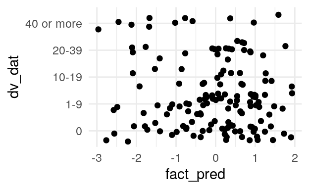
| lhs | op | rhs | est.std | se | z | pvalue | ci.lower | ci.upper |
|---|---|---|---|---|---|---|---|---|
| ordered_sex_freq | ~ | fsmi_mate | -0.11 | 0.08 | -1.36 | 0.17 | -0.26 | 0.05 |
| ordered_sex_freq | ~ | gender_c | -0.22 | 0.08 | -2.64 | 0.01 | -0.38 | -0.06 |
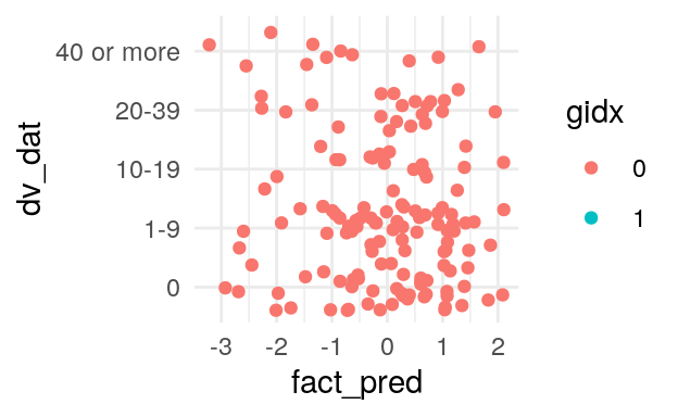
| lhs | op | rhs | group | est.std | se | z | pvalue | ci.lower | ci.upper |
|---|---|---|---|---|---|---|---|---|---|
| ordered_sex_freq | ~ | fsmi_mate | 1 | -0.11 | 0.08 | -1.30 | 0.19 | -0.26 | 0.05 |
| ordered_sex_freq | ~ | gender_c | 1 | -0.22 | 0.08 | -2.64 | 0.01 | -0.38 | -0.06 |
| ordered_sex_freq | ~ | fsmi_mate | 2 | -0.06 | 0.15 | -0.39 | 0.69 | -0.36 | 0.24 |
| ordered_sex_freq | ~ | gender_c | 2 | -0.03 | 0.16 | -0.16 | 0.88 | -0.34 | 0.29 |
| lhs | op | rhs | est.std | se | z | pvalue | ci.lower | ci.upper |
|---|---|---|---|---|---|---|---|---|
| ordered_sex_freq | ~ | neg_urgency | 0.22 | 0.21 | 1.06 | 0.29 | -0.19 | 0.63 |
| ordered_sex_freq | ~ | sensation_seeking | 0.13 | 0.11 | 1.20 | 0.23 | -0.08 | 0.34 |
| ordered_sex_freq | ~ | pos_urgency | -0.06 | 0.22 | -0.29 | 0.77 | -0.48 | 0.36 |
| ordered_sex_freq | ~ | fsmi_mate | 0.00 | 0.00 | 0.00 | 0.00 | ||
| ordered_sex_freq | ~ | gender_c | -0.17 | 0.10 | -1.80 | 0.07 | -0.36 | 0.02 |
| lhs | op | rhs | est.std | se | z | pvalue | ci.lower | ci.upper |
|---|---|---|---|---|---|---|---|---|
| ordered_sex_freq | ~ | neg_urgency | 0.25 | 0.20 | 1.25 | 0.21 | -0.15 | 0.65 |
| ordered_sex_freq | ~ | sensation_seeking | 0.15 | 0.11 | 1.42 | 0.16 | -0.06 | 0.36 |
| ordered_sex_freq | ~ | pos_urgency | -0.02 | 0.21 | -0.08 | 0.94 | -0.43 | 0.39 |
| ordered_sex_freq | ~ | fsmi_mate | -0.23 | 0.09 | -2.44 | 0.01 | -0.41 | -0.04 |
| ordered_sex_freq | ~ | gender_c | -0.17 | 0.10 | -1.80 | 0.07 | -0.36 | 0.02 |
| lhs | op | rhs | est.std | se | z | pvalue | ci.lower | ci.upper |
|---|---|---|---|---|---|---|---|---|
| ordered_sex_freq | ~ | neg_urgency | 0.30 | 0.18 | 1.68 | 0.09 | -0.05 | 0.64 |
| ordered_sex_freq | ~ | sensation_seeking | 0.10 | 0.09 | 1.16 | 0.24 | -0.07 | 0.28 |
| ordered_sex_freq | ~ | pos_urgency | -0.10 | 0.19 | -0.51 | 0.61 | -0.47 | 0.27 |
| ordered_sex_freq | ~ | fsmi_mate | -0.41 | 0.08 | -5.11 | 0.00 | -0.56 | -0.25 |
| ordered_sex_freq | ~ | gender_c | -0.12 | 0.09 | -1.35 | 0.18 | -0.29 | 0.05 |
There is not a strong association between FSMI Mate-seeking and number of sexual encounters in the past six months for unpartnered college students. The association was not examined in partnered college students because the Mate-seeking scale asks about looking for new romantic or sexual partners, and so (in normatively monogamous relationships) should not be theoretically related to frequency of sex.
K-SRQ sexual relationships
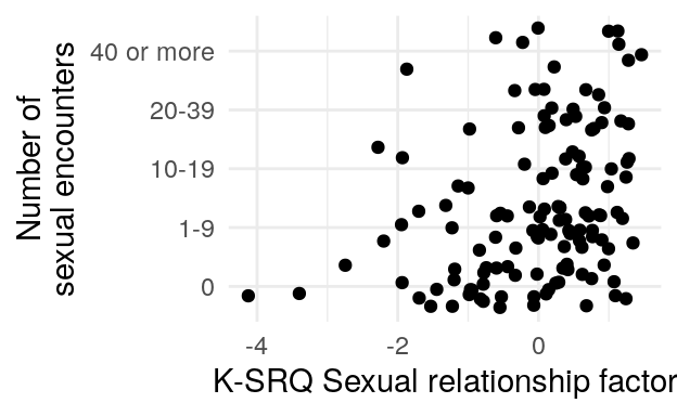
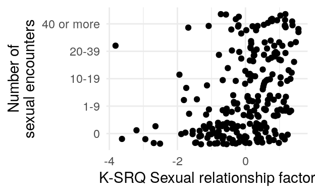
#> Scaled Chi Square Difference Test (method = "satorra.2000")
#>
#>                            Df AIC BIC  Chisq Chisq diff Df diff Pr(>Chisq)
#> ksrq_noadmrtn_sex_freq_sem 84         48.602
#> ksrq_sex_freq_null_sem     85         83.456     7.3583       1   0.006675 **
#> ---
#> Signif. codes:  0 '***' 0.001 '**' 0.01 '*' 0.05 '.' 0.1 ' ' 1
#> Scaled Chi Square Difference Test (method = "satorra.2000")
#>
#>                                Df AIC BIC  Chisq Chisq diff Df diff Pr(>Chisq)
#> ksrq_noadmrtn_sex_freq_all_sem 97         146.04
#> ksrq_sex_freq_null_all_sem     98         228.45     20.545       1  5.824e-06
#>
#> ksrq_noadmrtn_sex_freq_all_sem
#> ksrq_sex_freq_null_all_sem     ***
#> ---
#> Signif. codes:  0 '***' 0.001 '**' 0.01 '*' 0.05 '.' 0.1 ' ' 1
#> Scaled Chi Square Difference Test (method = "satorra.2000")
#>
#>                            Df AIC BIC  Chisq Chisq diff Df diff Pr(>Chisq)
#> ksrq_sex_freq_sem          83         46.868
#> ksrq_noadmrtn_sex_freq_sem 84         48.602      1.385       1     0.2392
#> Scaled Chi Square Difference Test (method = "satorra.2000")
#>
#>                                Df AIC BIC  Chisq Chisq diff Df diff Pr(>Chisq)
#> ksrq_sex_freq_all_sem          96         138.44
#> ksrq_noadmrtn_sex_freq_all_sem 97         146.04     6.8893       1   0.008671
#>
#> ksrq_sex_freq_all_sem
#> ksrq_noadmrtn_sex_freq_all_sem **
#> ---
#> Signif. codes:  0 '***' 0.001 '**' 0.01 '*' 0.05 '.' 0.1 ' ' 1
#> Scaled Chi Square Difference Test (method = "satorra.2000")
#>
#>                                Df AIC BIC  Chisq Chisq diff Df diff Pr(>Chisq)
#> uppsp_ksrq_sex_freq_sem      1301         1520.8
#> uppsp_ksrq_nosr_sex_freq_sem 1302         1524.9      1.945       1     0.1631
#> Scaled Chi Square Difference Test (method = "satorra.2000")
#>
#>                                     Df AIC BIC  Chisq Chisq diff Df diff
#> uppsp_ksrq_sex_freq_all__sem      1352         2069.4
#> uppsp_ksrq_nosr_sex_freq_all__sem 1353         2084.6     10.572       1
#>                                   Pr(>Chisq)
#> uppsp_ksrq_sex_freq_all__sem
#> uppsp_ksrq_nosr_sex_freq_all__sem   0.001148 **
#> ---
#> Signif. codes: 0 '***' 0.001 '**' 0.01 '*' 0.05 '.' 0.1 ' ' 1| lhs | op | rhs | est | se | z | pvalue | ci.lower | ci.upper | std.lv | std.all | std.nox |
|---|---|---|---|---|---|---|---|---|---|---|---|
| ordered_sex_freq | ~ | k_srq_sexual_relationships | 0.41 | 0.14 | 2.86 | 0.00 | 0.13 | 0.68 | 0.44 | 0.44 | 0.44 |
| ordered_sex_freq | ~ | k_srq_admiration | -0.18 | 0.15 | -1.19 | 0.23 | -0.47 | 0.12 | -0.19 | -0.19 | -0.19 |
| ordered_sex_freq | ~ | gender_c | -0.27 | 0.20 | -1.31 | 0.19 | -0.66 | 0.13 | -0.27 | -0.12 | -0.26 |
| lhs | op | rhs | est | se | z | pvalue | ci.lower | ci.upper | std.lv | std.all | std.nox |
|---|---|---|---|---|---|---|---|---|---|---|---|
| ordered_sex_freq | ~ | k_srq_sexual_relationships | 0.24 | 0.09 | 2.81 | 0.01 | 0.07 | 0.41 | 0.26 | 0.26 | 0.26 |
| ordered_sex_freq | ~ | k_srq_admiration | 0.00 | 0.00 | 0.00 | 0.00 | 0.00 | 0.00 | 0.00 | ||
| ordered_sex_freq | ~ | gender_c | -0.27 | 0.20 | -1.31 | 0.19 | -0.66 | 0.13 | -0.27 | -0.12 | -0.26 |
| lhs | op | rhs | est | se | z | pvalue | ci.lower | ci.upper | std.lv | std.all | std.nox |
|---|---|---|---|---|---|---|---|---|---|---|---|
| ordered_sex_freq | ~ | k_srq_sexual_relationships | 0.55 | 0.10 | 5.76 | 0.00 | 0.36 | 0.73 | 0.58 | 0.50 | 0.50 |
| ordered_sex_freq | ~ | k_srq_admiration | -0.31 | 0.11 | -2.68 | 0.01 | -0.53 | -0.08 | -0.28 | -0.24 | -0.24 |
| ordered_sex_freq | ~ | gender_c | 0.14 | 0.16 | 0.87 | 0.38 | -0.17 | 0.46 | 0.14 | 0.06 | 0.12 |
| ordered_sex_freq | ~ | age_c | 0.26 | 0.04 | 6.62 | 0.00 | 0.18 | 0.34 | 0.26 | 0.50 | 0.22 |
| lhs | op | rhs | est | se | z | pvalue | ci.lower | ci.upper | std.lv | std.all | std.nox |
|---|---|---|---|---|---|---|---|---|---|---|---|
| ordered_sex_freq | ~ | k_srq_sexual_relationships | 0.29 | 0.06 | 4.54 | 0.00 | 0.17 | 0.42 | 0.32 | 0.27 | 0.27 |
| ordered_sex_freq | ~ | k_srq_admiration | 0.00 | 0.00 | 0.00 | 0.00 | 0.00 | 0.00 | 0.00 | ||
| ordered_sex_freq | ~ | gender_c | 0.14 | 0.16 | 0.87 | 0.38 | -0.17 | 0.46 | 0.14 | 0.06 | 0.12 |
| ordered_sex_freq | ~ | age_c | 0.26 | 0.04 | 6.62 | 0.00 | 0.18 | 0.34 | 0.26 | 0.50 | 0.22 |
| lhs | op | rhs | est | se | z | pvalue | ci.lower | ci.upper | std.lv | std.all | std.nox |
|---|---|---|---|---|---|---|---|---|---|---|---|
| ordered_sex_freq | ~ | neg_urgency | 0.45 | 0.57 | 0.80 | 0.42 | -0.66 | 1.57 | 0.18 | 0.18 | 0.18 |
| ordered_sex_freq | ~ | sensation_seeking | 0.10 | 0.33 | 0.31 | 0.75 | -0.54 | 0.74 | 0.04 | 0.04 | 0.04 |
| ordered_sex_freq | ~ | pos_urgency | -0.10 | 0.41 | -0.25 | 0.81 | -0.90 | 0.70 | -0.05 | -0.05 | -0.05 |
| ordered_sex_freq | ~ | k_srq_sexual_relationships | 0.15 | 0.10 | 1.51 | 0.13 | -0.05 | 0.36 | 0.19 | 0.19 | 0.19 |
| ordered_sex_freq | ~ | gender_c | -0.27 | 0.22 | -1.26 | 0.21 | -0.70 | 0.15 | -0.27 | -0.13 | -0.27 |
| lhs | op | rhs | est | se | z | pvalue | ci.lower | ci.upper | std.lv | std.all | std.nox |
|---|---|---|---|---|---|---|---|---|---|---|---|
| ordered_sex_freq | ~ | neg_urgency | 1.31 | 0.66 | 1.99 | 0.05 | 0.02 | 2.59 | 0.52 | 0.51 | 0.51 |
| ordered_sex_freq | ~ | sensation_seeking | 0.39 | 0.30 | 1.30 | 0.19 | -0.20 | 0.99 | 0.16 | 0.16 | 0.16 |
| ordered_sex_freq | ~ | pos_urgency | -0.67 | 0.44 | -1.51 | 0.13 | -1.53 | 0.20 | -0.36 | -0.35 | -0.35 |
| ordered_sex_freq | ~ | k_srq_sexual_relationships | 0.00 | 0.00 | 0.00 | 0.00 | 0.00 | 0.00 | 0.00 | ||
| ordered_sex_freq | ~ | gender_c | -0.27 | 0.22 | -1.26 | 0.21 | -0.70 | 0.15 | -0.27 | -0.13 | -0.27 |
| lhs | op | rhs | est | se | z | pvalue | ci.lower | ci.upper | std.lv | std.all | std.nox |
|---|---|---|---|---|---|---|---|---|---|---|---|
| ordered_sex_freq | ~ | neg_urgency | 0.19 | 0.41 | 0.46 | 0.64 | -0.61 | 0.99 | 0.09 | 0.07 | 0.07 |
| ordered_sex_freq | ~ | sensation_seeking | 0.06 | 0.21 | 0.30 | 0.76 | -0.35 | 0.48 | 0.03 | 0.03 | 0.03 |
| ordered_sex_freq | ~ | pos_urgency | 0.04 | 0.31 | 0.13 | 0.90 | -0.57 | 0.65 | 0.02 | 0.02 | 0.02 |
| ordered_sex_freq | ~ | k_srq_sexual_relationships | 0.26 | 0.08 | 3.39 | 0.00 | 0.11 | 0.41 | 0.30 | 0.25 | 0.25 |
| ordered_sex_freq | ~ | gender_c | 0.14 | 0.18 | 0.80 | 0.42 | -0.20 | 0.48 | 0.14 | 0.06 | 0.12 |
| ordered_sex_freq | ~ | age_c | 0.27 | 0.04 | 6.45 | 0.00 | 0.19 | 0.35 | 0.27 | 0.51 | 0.23 |
| lhs | op | rhs | est | se | z | pvalue | ci.lower | ci.upper | std.lv | std.all | std.nox |
|---|---|---|---|---|---|---|---|---|---|---|---|
| ordered_sex_freq | ~ | neg_urgency | 2.02 | 0.60 | 3.36 | 0.00 | 0.84 | 3.21 | 0.91 | 0.78 | 0.78 |
| ordered_sex_freq | ~ | sensation_seeking | 0.39 | 0.21 | 1.84 | 0.07 | -0.03 | 0.80 | 0.18 | 0.16 | 0.16 |
| ordered_sex_freq | ~ | pos_urgency | -1.31 | 0.41 | -3.17 | 0.00 | -2.11 | -0.50 | -0.79 | -0.68 | -0.68 |
| ordered_sex_freq | ~ | k_srq_sexual_relationships | 0.00 | 0.00 | 0.00 | 0.00 | 0.00 | 0.00 | 0.00 | ||
| ordered_sex_freq | ~ | gender_c | 0.14 | 0.18 | 0.80 | 0.42 | -0.20 | 0.48 | 0.14 | 0.06 | 0.12 |
| ordered_sex_freq | ~ | age_c | 0.27 | 0.04 | 6.45 | 0.00 | 0.19 | 0.35 | 0.27 | 0.51 | 0.23 |
K-SRQ Sexual Relationships is associated with number of sexual partners when considering the full sample, and the sign and size of the coefficient is similar when considering only the unpartnered college sample. Again, Sociability and Sexual Relationships are too highly correlated to be disentangled. Controlling for the other highly correlated K-SRQ scale, Admiration, yields a standardized effect of Sexual Relationships that has the same sign, but that has bigger magnitude. As above, the coefficient for the Admiration scale is large and negative when controlling for K-SRQ Sexual Relationships.
SPLT parameters
#> Scaled Chi Square Difference Test (method = "satorra.2000")
#>
#>                        Df AIC BIC   Chisq Chisq diff Df diff Pr(>Chisq)
#> splt_sex_freq_sem       9          3.3479
#> splt_sex_freq_null_sem 10         12.7942     3.2935       1    0.06956 .
#> ---
#> Signif. codes:  0 '***' 0.001 '**' 0.01 '*' 0.05 '.' 0.1 ' ' 1
#> Scaled Chi Square Difference Test (method = "satorra.2000")
#>
#>                            Df AIC BIC  Chisq Chisq diff Df diff Pr(>Chisq)
#> splt_sex_freq_all_sem      14         21.087
#> splt_sex_freq_all_null_sem 15         22.643    0.58162       1     0.4457
#> Scaled Chi Square Difference Test (method = "satorra.2000")
#>
#>                        Df AIC BIC   Chisq Chisq diff Df diff Pr(>Chisq)
#> splt_sex_freq_sem       9          5.9599
#> splt_sex_freq_null_sem 10         11.3797     1.2813       1     0.2577
#> Scaled Chi Square Difference Test (method = "satorra.2000")
#>
#>                            Df AIC BIC   Chisq Chisq diff Df diff Pr(>Chisq)
#> splt_sex_freq_all_sem      14          9.4307
#> splt_sex_freq_all_null_sem 15         10.7133    0.31229       1     0.5763
#> Scaled Chi Square Difference Test (method = "satorra.2000")
#>
#>                        Df AIC BIC  Chisq Chisq diff Df diff Pr(>Chisq)
#> splt_sex_freq_sem       9         16.387
#> splt_sex_freq_null_sem 10         16.612     0.1305       1     0.7179
#> Scaled Chi Square Difference Test (method = "satorra.2000")
#>
#>                            Df AIC BIC  Chisq Chisq diff Df diff Pr(>Chisq)
#> splt_sex_freq_all_sem      14         10.952
#> splt_sex_freq_all_null_sem 15         10.981   0.017396       1     0.8951
#> Scaled Chi Square Difference Test (method = "satorra.2000")
#>
#>                        Df AIC BIC  Chisq Chisq diff Df diff Pr(>Chisq)
#> splt_sex_freq_sem       9         2.4562
#> splt_sex_freq_null_sem 10         3.1952     0.3417       1     0.5588
#> Scaled Chi Square Difference Test (method = "satorra.2000")
#>
#>                            Df AIC BIC  Chisq Chisq diff Df diff Pr(>Chisq)
#> splt_sex_freq_all_sem      14         5.4056
#> splt_sex_freq_all_null_sem 15         5.9869     0.2494       1     0.6175
#> Scaled Chi Square Difference Test (method = "satorra.2000")
#>
#>                        Df AIC BIC  Chisq Chisq diff Df diff Pr(>Chisq)
#> splt_sex_freq_sem       9         7.1147
#> splt_sex_freq_null_sem 10         7.4313     0.1671       1     0.6827
#> Scaled Chi Square Difference Test (method = "satorra.2000")
#>
#>                            Df AIC BIC  Chisq Chisq diff Df diff Pr(>Chisq)
#> splt_sex_freq_all_sem      14         19.096
#> splt_sex_freq_all_null_sem 15         22.973     1.9504       1     0.1625
#> Scaled Chi Square Difference Test (method = "satorra.2000")
#>
#>                        Df AIC BIC  Chisq Chisq diff Df diff Pr(>Chisq)
#> splt_sex_freq_sem       9         5.9843
#> splt_sex_freq_null_sem 10         7.6761    0.87526       1     0.3495
#> Scaled Chi Square Difference Test (method = "satorra.2000")
#>
#>                            Df AIC BIC   Chisq Chisq diff Df diff Pr(>Chisq)
#> splt_sex_freq_all_sem      14          9.3549
#> splt_sex_freq_all_null_sem 15         11.0476     0.9379       1     0.3328
#>
#>
#> Table: (\#tab:unnamed-chunk-56)$\epsilon$ predicting number of partners among unpartnered college students; N obs. = 151
#>
#> lhs                op   rhs                       est     se       z   pvalue   ci.lower   ci.upper   std.lv   std.all   std.nox
#> -----------------  ---  ---------------------  ------  -----  ------  -------  ---------  ---------  -------  --------  --------
#> ordered_sex_freq   ~    ep_prm_DtngLHngT_fac    -2.68   1.43   -1.87     0.06      -5.49       0.13    -0.17     -0.17     -0.17
#> ordered_sex_freq   ~    gender_c                -0.40   0.19   -2.12     0.03      -0.77      -0.03    -0.40     -0.18     -0.39
#>
#>
#> Table: (\#tab:unnamed-chunk-56)$\epsilon$ predicting number of partners among all adolescent and college participants with SES responses; N obs. = 260
#>
#> lhs                op   rhs                       est     se       z   pvalue   ci.lower   ci.upper   std.lv   std.all   std.nox
#> -----------------  ---  ---------------------  ------  -----  ------  -------  ---------  ---------  -------  --------  --------
#> ordered_sex_freq   ~    ep_prm_DtngLHngT_fac    -0.90   1.17   -0.77     0.44      -3.18       1.39    -0.05     -0.05     -0.05
#> ordered_sex_freq   ~    gender_c                 0.00   0.15    0.01     0.99      -0.30       0.30     0.00      0.00      0.00
#> ordered_sex_freq   ~    age_c                    0.24   0.04    6.37     0.00       0.17       0.32     0.24      0.46      0.22
#>
#>
#> Table: (\#tab:unnamed-chunk-56)$\rho$ predicting number of partners among unpartnered college students; N obs. = 151
#>
#> lhs                op   rhs                        est     se       z   pvalue   ci.lower   ci.upper   std.lv   std.all   std.nox
#> -----------------  ---  ----------------------  ------  -----  ------  -------  ---------  ---------  -------  --------  --------
#> ordered_sex_freq   ~    rho_prm_DtngLHngT_fac    -0.13   0.11   -1.14     0.25      -0.36       0.09    -0.09     -0.09     -0.09
#> ordered_sex_freq   ~    gender_c                 -0.40   0.19   -2.12     0.03      -0.77      -0.03    -0.40     -0.18     -0.39
#>
#>
#> Table: (\#tab:unnamed-chunk-56)$\rho$ predicting number of partners among all adolescent and college participants with SES responses; N obs. = 260
#>
#> lhs                op   rhs                       est     se      z   pvalue   ci.lower   ci.upper   std.lv   std.all   std.nox
#> -----------------  ---  ----------------------  -----  -----  -----  -------  ---------  ---------  -------  --------  --------
#> ordered_sex_freq   ~    rho_prm_DtngLHngT_fac    0.06   0.11   0.56     0.58      -0.15       0.28     0.04      0.03      0.03
#> ordered_sex_freq   ~    gender_c                 0.00   0.15   0.01     0.99      -0.30       0.30     0.00      0.00      0.00
#> ordered_sex_freq   ~    age_c                    0.24   0.04   6.37     0.00       0.17       0.32     0.24      0.46      0.22
#>
#>
#> Table: (\#tab:unnamed-chunk-56)$\xi$ predicting number of partners among unpartnered college students; N obs. = 151
#>
#> lhs                op   rhs                      est     se       z   pvalue   ci.lower   ci.upper   std.lv   std.all   std.nox
#> -----------------  ---  ---------------------  -----  -----  ------  -------  ---------  ---------  -------  --------  --------
#> ordered_sex_freq   ~    xi_prm_DtngLHngT_fac     0.4   1.09    0.36     0.72      -1.75       2.54     0.03      0.03      0.03
#> ordered_sex_freq   ~    gender_c                -0.4   0.19   -2.12     0.03      -0.77      -0.03    -0.40     -0.18     -0.39
#>
#>
#> Table: (\#tab:unnamed-chunk-56)$\xi$ predicting number of partners among all adolescent and college participants with SES responses; N obs. = 260
#>
#> lhs                op   rhs                      est     se      z   pvalue   ci.lower   ci.upper   std.lv   std.all   std.nox
#> -----------------  ---  ---------------------  -----  -----  -----  -------  ---------  ---------  -------  --------  --------
#> ordered_sex_freq   ~    xi_prm_DtngLHngT_fac    0.13   0.96   0.13     0.90      -1.76       2.02     0.01      0.01      0.01
#> ordered_sex_freq   ~    gender_c                0.00   0.15   0.01     0.99      -0.30       0.30     0.00      0.00      0.00
#> ordered_sex_freq   ~    age_c                   0.24   0.04   6.37     0.00       0.17       0.32     0.24      0.46      0.22
#>
#>
#> Table: (\#tab:unnamed-chunk-56)$b$ predicting number of partners among unpartnered college students; N obs. = 151
#>
#> lhs                op   rhs                  est     se       z   pvalue   ci.lower   ci.upper   std.lv   std.all   std.nox
#> -----------------  ---  ----------------  ------  -----  ------  -------  ---------  ---------  -------  --------  --------
#> ordered_sex_freq   ~    b_DtngLHngT_fac     0.19   0.33    0.58     0.56      -0.45       0.83     0.05      0.05      0.05
#> ordered_sex_freq   ~    gender_c           -0.40   0.19   -2.12     0.03      -0.77      -0.03    -0.40     -0.18     -0.39
#>
#>
#> Table: (\#tab:unnamed-chunk-56)$b$ predicting number of partners among all adolescent and college participants with SES responses; N obs. = 260
#>
#> lhs                op   rhs                 est     se      z   pvalue   ci.lower   ci.upper   std.lv   std.all   std.nox
#> -----------------  ---  ----------------  -----  -----  -----  -------  ---------  ---------  -------  --------  --------
#> ordered_sex_freq   ~    b_DtngLHngT_fac    0.12   0.23   0.50     0.62      -0.34       0.57     0.03      0.03      0.03
#> ordered_sex_freq   ~    gender_c           0.00   0.15   0.01     0.99      -0.30       0.30     0.00      0.00      0.00
#> ordered_sex_freq   ~    age_c              0.24   0.04   6.37     0.00       0.17       0.32     0.24      0.46      0.22
#>
#>
#> Table: (\#tab:unnamed-chunk-56)First-half optimal responses predicting number of partners among unpartnered college students; N obs. = 151
#>
#> lhs                op   rhs                               est     se       z   pvalue   ci.lower   ci.upper   std.lv   std.all   std.nox
#> -----------------  ---  -----------------------------  ------  -----  ------  -------  ---------  ---------  -------  --------  --------
#> ordered_sex_freq   ~    bin_start_to_4_DtngLHngT_fac    -0.23   0.55   -0.41     0.68      -1.31       0.86    -0.03     -0.03     -0.03
#> ordered_sex_freq   ~    gender_c                        -0.40   0.19   -2.12     0.03      -0.77      -0.03    -0.40     -0.18     -0.39
#>
#>
#> Table: (\#tab:unnamed-chunk-56)First-half optimal responses predicting number of partners among all adolescent and college participants with SES responses; N obs. = 260
#>
#> lhs                op   rhs                              est     se      z   pvalue   ci.lower   ci.upper   std.lv   std.all   std.nox
#> -----------------  ---  -----------------------------  -----  -----  -----  -------  ---------  ---------  -------  --------  --------
#> ordered_sex_freq   ~    bin_start_to_4_DtngLHngT_fac    0.63   0.45   1.41     0.16      -0.25       1.51     0.09      0.08      0.08
#> ordered_sex_freq   ~    gender_c                        0.00   0.15   0.01     0.99      -0.30       0.30     0.00      0.00      0.00
#> ordered_sex_freq   ~    age_c                           0.24   0.04   6.37     0.00       0.17       0.32     0.24      0.46      0.22
#>
#>
#> Table: (\#tab:unnamed-chunk-56)Last-half optimal responses predicting number of partners among unpartnered college students; N obs. = 151
#>
#> lhs                op   rhs                             est     se       z   pvalue   ci.lower   ci.upper   std.lv   std.all   std.nox
#> -----------------  ---  ---------------------------  ------  -----  ------  -------  ---------  ---------  -------  --------  --------
#> ordered_sex_freq   ~    bin_5_to_end_DtngLHngT_fac    -0.53   0.56   -0.94     0.35      -1.62       0.57    -0.08     -0.08     -0.08
#> ordered_sex_freq   ~    gender_c                      -0.40   0.19   -2.12     0.03      -0.77      -0.03    -0.40     -0.18     -0.39
#>
#>
#> Table: (\#tab:unnamed-chunk-56)Last-half optimal responses predicting number of partners among all adolescent and college participants with SES responses; N obs. = 260
#>
#> lhs                op   rhs                             est     se       z   pvalue   ci.lower   ci.upper   std.lv   std.all   std.nox
#> -----------------  ---  ---------------------------  ------  -----  ------  -------  ---------  ---------  -------  --------  --------
#> ordered_sex_freq   ~    bin_5_to_end_DtngLHngT_fac    -0.47   0.48   -0.97     0.33      -1.41       0.48    -0.07     -0.06     -0.06
#> ordered_sex_freq   ~    gender_c                       0.00   0.15    0.01     0.99      -0.30       0.30     0.00      0.00      0.00
#> ordered_sex_freq   ~    age_c                          0.24   0.04    6.37     0.00       0.17       0.32     0.24      0.46      0.22
Again, no \(\chi^2\) tests satisfy the \(\alpha = .005\) cutoff. The biggest association is with the \(\epsilon\) contrast variable, but it has the wrong sign, with higher learning rates being associated with fewer sexual encounters.
Health-related behavior
Using protection
FSMI mate seeking
#> Chi Square Difference Test
#>
#>                              Df    AIC    BIC  Chisq Chisq diff Df diff
#> fsmi_use_protection_sem      76 7414.4 7541.5 106.51
#> fsmi_use_protection_null_sem 77 7412.4 7536.4 106.51   0.001217       1
#>                              Pr(>Chisq)
#> fsmi_use_protection_sem
#> fsmi_use_protection_null_sem     0.9722
#> Chi Square Difference Test
#>
#>                                  Df   AIC   BIC  Chisq Chisq diff Df diff
#> fsmi_use_protection_all_sem      76 10375 10515 111.75
#> fsmi_use_protection_all_null_sem 77 10373 10510 111.77     0.0152       1
#>                                  Pr(>Chisq)
#> fsmi_use_protection_all_sem
#> fsmi_use_protection_all_null_sem     0.9019
#> Chi Square Difference Test
#>
#>                              Df   AIC   BIC  Chisq Chisq diff Df diff
#> uppsp_fsmi_uprot_sem        980 16217 16666 1830.9
#> uppsp_fsmi_uprot_noupps_sem 983 16216 16656 1836.4     5.4646       3
#> uppsp_fsmi_uprot_null_sem   984 16214 16651 1836.4     0.0006       1
#>                             Pr(>Chisq)
#> uppsp_fsmi_uprot_sem
#> uppsp_fsmi_uprot_noupps_sem     0.1408
#> uppsp_fsmi_uprot_null_sem       0.9810
#> Chi Square Difference Test
#>
#>                              Df   AIC   BIC  Chisq Chisq diff Df diff
#> uppsp_fsmi_uprot_sem        980 16217 16666 1830.9
#> uppsp_fsmi_uprot_nofsmi_sem 981 16215 16661 1831.4     0.4270       1
#> uppsp_fsmi_uprot_null_sem   984 16214 16651 1836.4     5.0382       3
#>                             Pr(>Chisq)
#> uppsp_fsmi_uprot_sem
#> uppsp_fsmi_uprot_nofsmi_sem     0.5135
#> uppsp_fsmi_uprot_null_sem       0.1690
#> Chi Square Difference Test
#>
#>                              Df   AIC   BIC  Chisq Chisq diff Df diff
#> uppsp_fsmi_uprot_sem        980 16217 16666 1830.9
#> uppsp_fsmi_uprot_nopurg_sem 981 16215 16661 1830.9     0.0024       1
#> uppsp_fsmi_uprot_null_sem   984 16214 16651 1836.4     5.4628       3
#>                             Pr(>Chisq)
#> uppsp_fsmi_uprot_sem
#> uppsp_fsmi_uprot_nopurg_sem     0.9613
#> uppsp_fsmi_uprot_null_sem       0.1409
#> Chi Square Difference Test
#>
#>                              Df   AIC   BIC  Chisq Chisq diff Df diff
#> uppsp_fsmi_uprot_sem        980 16217 16666 1830.9
#> uppsp_fsmi_uprot_nonurg_sem 981 16216 16662 1832.1     1.2084       1
#> uppsp_fsmi_uprot_null_sem   984 16214 16651 1836.4     4.2567       3
#>                             Pr(>Chisq)
#> uppsp_fsmi_uprot_sem
#> uppsp_fsmi_uprot_nonurg_sem     0.2716
#> uppsp_fsmi_uprot_null_sem       0.2350
#> Chi Square Difference Test
#>
#>                            Df   AIC   BIC  Chisq Chisq diff Df diff Pr(>Chisq)
#> uppsp_fsmi_uprot_sem      980 16217 16666 1830.9
#> uppsp_fsmi_uprot_noss_sem 981 16216 16662 1832.4     1.5169       1     0.2181
#> uppsp_fsmi_uprot_null_sem 984 16214 16651 1836.4     3.9482       3     0.2671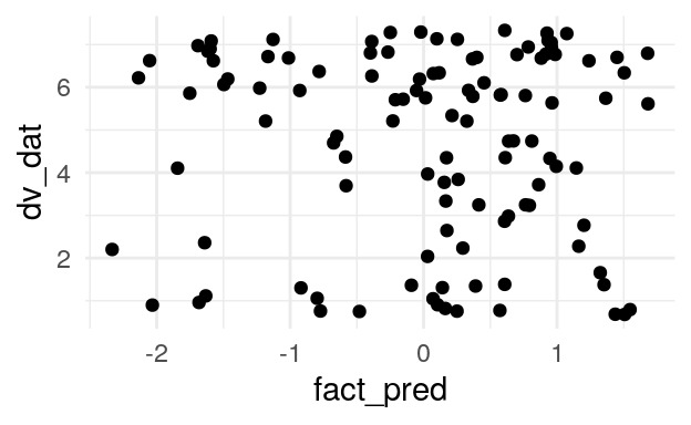
| lhs | op | rhs | est.std | se | z | pvalue | ci.lower | ci.upper |
|---|---|---|---|---|---|---|---|---|
| continuous_use_protection | ~ | fsmi_mate | 0.00 | 0.10 | -0.03 | 0.97 | -0.20 | 0.19 |
| continuous_use_protection | ~ | gender_c | 0.16 | 0.09 | 1.84 | 0.07 | -0.01 | 0.34 |
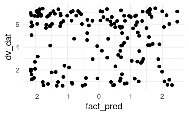
| lhs | op | rhs | est.std | se | z | pvalue | ci.lower | ci.upper |
|---|---|---|---|---|---|---|---|---|
| continuous_use_protection | ~ | fsmi_mate | -0.01 | 0.08 | -0.12 | 0.90 | -0.16 | 0.15 |
| continuous_use_protection | ~ | gender_c | 0.14 | 0.07 | 1.81 | 0.07 | -0.01 | 0.28 |
| lhs | op | rhs | est.std | se | z | pvalue | ci.lower | ci.upper |
|---|---|---|---|---|---|---|---|---|
| continuous_use_protection | ~ | neg_urgency | 0.17 | 0.17 | 1.03 | 0.30 | -0.16 | 0.50 |
| continuous_use_protection | ~ | sensation_seeking | 0.13 | 0.11 | 1.22 | 0.22 | -0.08 | 0.35 |
| continuous_use_protection | ~ | pos_urgency | -0.01 | 0.17 | -0.08 | 0.94 | -0.35 | 0.32 |
| continuous_use_protection | ~ | fsmi_mate | 0.00 | 0.00 | 0.00 | 0.00 | ||
| continuous_use_protection | ~ | gender_c | 0.20 | 0.09 | 2.29 | 0.02 | 0.03 | 0.36 |
| lhs | op | rhs | est.std | se | z | pvalue | ci.lower | ci.upper |
|---|---|---|---|---|---|---|---|---|
| continuous_use_protection | ~ | neg_urgency | 0.19 | 0.17 | 1.11 | 0.27 | -0.14 | 0.52 |
| continuous_use_protection | ~ | sensation_seeking | 0.14 | 0.11 | 1.25 | 0.21 | -0.08 | 0.35 |
| continuous_use_protection | ~ | pos_urgency | -0.01 | 0.17 | -0.05 | 0.96 | -0.34 | 0.33 |
| continuous_use_protection | ~ | fsmi_mate | -0.07 | 0.10 | -0.65 | 0.51 | -0.26 | 0.13 |
| continuous_use_protection | ~ | gender_c | 0.19 | 0.09 | 2.20 | 0.03 | 0.02 | 0.36 |
| lhs | op | rhs | est.std | se | z | pvalue | ci.lower | ci.upper |
|---|---|---|---|---|---|---|---|---|
| continuous_use_protection | ~ | neg_urgency | 0.16 | 0.15 | 1.08 | 0.28 | -0.13 | 0.44 |
| continuous_use_protection | ~ | sensation_seeking | 0.05 | 0.09 | 0.50 | 0.61 | -0.13 | 0.23 |
| continuous_use_protection | ~ | pos_urgency | 0.02 | 0.15 | 0.13 | 0.90 | -0.27 | 0.31 |
| continuous_use_protection | ~ | fsmi_mate | -0.07 | 0.08 | -0.85 | 0.39 | -0.23 | 0.09 |
| continuous_use_protection | ~ | gender_c | 0.16 | 0.08 | 2.08 | 0.04 | 0.01 | 0.30 |
There estimate of the association between FSMI Mate-seeking and safe sex practices for unpartnered college students is very close to 0 (\(\beta = -0.003\), 95% CI = [-0.20,0.19]). Fixing the coefficient for this association to 0 did not result in significant reduction in fit in any model specification
K-SRQ sexual relationships
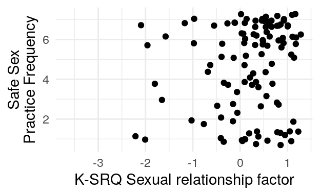
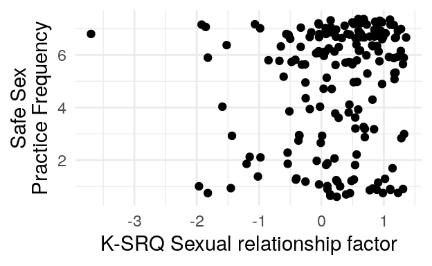
#> Chi Square Difference Test
#>
#>                                  Df    AIC    BIC  Chisq Chisq diff Df diff
#> ksrq_noadmrtn_use_protection_sem 84 7195.3 7347.2 134.06
#> ksrq_use_protection_null_sem     85 7194.9 7343.7 135.68     1.6163       1
#>                                  Pr(>Chisq)
#> ksrq_noadmrtn_use_protection_sem
#> ksrq_use_protection_null_sem         0.2036
#> Chi Square Difference Test
#>
#>                                      Df   AIC   BIC  Chisq Chisq diff Df diff
#> ksrq_noadmrtn_use_protection_all_sem 97 16002 16192 250.90
#> ksrq_use_protection_null_all_sem     98 16001 16188 252.23     1.3253       1
#>                                      Pr(>Chisq)
#> ksrq_noadmrtn_use_protection_all_sem
#> ksrq_use_protection_null_all_sem         0.2496
#> Chi Square Difference Test
#>
#>                                  Df    AIC    BIC  Chisq Chisq diff Df diff
#> ksrq_use_protection_sem          83 7197.1 7352.0 133.84
#> ksrq_noadmrtn_use_protection_sem 84 7195.3 7347.2 134.06    0.22592       1
#>                                  Pr(>Chisq)
#> ksrq_use_protection_sem
#> ksrq_noadmrtn_use_protection_sem     0.6346
#> Chi Square Difference Test
#>
#>                                      Df   AIC   BIC Chisq Chisq diff Df diff
#> ksrq_use_protection_all_sem          96 16004 16198 250.7
#> ksrq_noadmrtn_use_protection_all_sem 97 16002 16192 250.9    0.19844       1
#>                                      Pr(>Chisq)
#> ksrq_use_protection_all_sem
#> ksrq_noadmrtn_use_protection_all_sem      0.656
#> Chi Square Difference Test
#>
#>                                      Df   AIC   BIC  Chisq Chisq diff Df diff
#> uppsp_ksrq_use_protection_sem      1301 19200 19762 2200.3
#> uppsp_ksrq_nosr_use_protection_sem 1302 19199 19757 2200.5    0.15768       1
#>                                    Pr(>Chisq)
#> uppsp_ksrq_use_protection_sem
#> uppsp_ksrq_nosr_use_protection_sem     0.6913
#> Chi Square Difference Test
#>
#>                                           Df   AIC   BIC  Chisq Chisq diff
#> uppsp_ksrq_use_protection_all__sem      1352 41662 42355 2906.5
#> uppsp_ksrq_nosr_use_protection_all__sem 1353 41660 42349 2907.2    0.63114
#>                                         Df diff Pr(>Chisq)
#> uppsp_ksrq_use_protection_all__sem
#> uppsp_ksrq_nosr_use_protection_all__sem 1 0.4269| lhs | op | rhs | est.std | se | z | pvalue | ci.lower | ci.upper |
|---|---|---|---|---|---|---|---|---|
| continuous_use_protection | ~ | k_srq_sexual_relationships | 0.09 | 0.17 | 0.50 | 0.61 | -0.25 | 0.43 |
| continuous_use_protection | ~ | k_srq_admiration | 0.07 | 0.15 | 0.48 | 0.63 | -0.22 | 0.37 |
| continuous_use_protection | ~ | gender_c | 0.17 | 0.09 | 1.94 | 0.05 | 0.00 | 0.34 |
| lhs | op | rhs | est.std | se | z | pvalue | ci.lower | ci.upper |
|---|---|---|---|---|---|---|---|---|
| continuous_use_protection | ~ | k_srq_sexual_relationships | 0.15 | 0.12 | 1.29 | 0.20 | -0.08 | 0.38 |
| continuous_use_protection | ~ | k_srq_admiration | 0.00 | 0.00 | 0.00 | 0.00 | ||
| continuous_use_protection | ~ | gender_c | 0.17 | 0.09 | 1.95 | 0.05 | 0.00 | 0.34 |
| lhs | op | rhs | est.std | se | z | pvalue | ci.lower | ci.upper |
|---|---|---|---|---|---|---|---|---|
| continuous_use_protection | ~ | k_srq_sexual_relationships | 0.06 | 0.15 | 0.40 | 0.69 | -0.23 | 0.35 |
| continuous_use_protection | ~ | k_srq_admiration | 0.06 | 0.13 | 0.45 | 0.66 | -0.19 | 0.30 |
| continuous_use_protection | ~ | gender_c | 0.13 | 0.08 | 1.70 | 0.09 | -0.02 | 0.28 |
| continuous_use_protection | ~ | age_c | -0.08 | 0.11 | -0.74 | 0.46 | -0.29 | 0.13 |
| lhs | op | rhs | est.std | se | z | pvalue | ci.lower | ci.upper |
|---|---|---|---|---|---|---|---|---|
| continuous_use_protection | ~ | k_srq_sexual_relationships | 0.11 | 0.09 | 1.16 | 0.25 | -0.07 | 0.29 |
| continuous_use_protection | ~ | k_srq_admiration | 0.00 | 0.00 | 0.00 | 0.00 | ||
| continuous_use_protection | ~ | gender_c | 0.13 | 0.08 | 1.70 | 0.09 | -0.02 | 0.28 |
| continuous_use_protection | ~ | age_c | -0.09 | 0.11 | -0.80 | 0.43 | -0.30 | 0.13 |
| lhs | op | rhs | est.std | se | z | pvalue | ci.lower | ci.upper |
|---|---|---|---|---|---|---|---|---|
| continuous_use_protection | ~ | neg_urgency | 0.14 | 0.19 | 0.75 | 0.46 | -0.23 | 0.52 |
| continuous_use_protection | ~ | sensation_seeking | 0.10 | 0.12 | 0.81 | 0.42 | -0.14 | 0.35 |
| continuous_use_protection | ~ | pos_urgency | 0.02 | 0.18 | 0.10 | 0.92 | -0.34 | 0.38 |
| continuous_use_protection | ~ | k_srq_sexual_relationships | 0.06 | 0.15 | 0.40 | 0.69 | -0.23 | 0.34 |
| continuous_use_protection | ~ | gender_c | 0.20 | 0.09 | 2.28 | 0.02 | 0.03 | 0.36 |
| lhs | op | rhs | est.std | se | z | pvalue | ci.lower | ci.upper |
|---|---|---|---|---|---|---|---|---|
| continuous_use_protection | ~ | neg_urgency | 0.18 | 0.17 | 1.08 | 0.28 | -0.15 | 0.51 |
| continuous_use_protection | ~ | sensation_seeking | 0.13 | 0.11 | 1.16 | 0.25 | -0.09 | 0.34 |
| continuous_use_protection | ~ | pos_urgency | -0.01 | 0.17 | -0.08 | 0.93 | -0.34 | 0.31 |
| continuous_use_protection | ~ | k_srq_sexual_relationships | 0.00 | 0.00 | 0.00 | 0.00 | ||
| continuous_use_protection | ~ | gender_c | 0.20 | 0.09 | 2.29 | 0.02 | 0.03 | 0.36 |
| lhs | op | rhs | est.std | se | z | pvalue | ci.lower | ci.upper |
|---|---|---|---|---|---|---|---|---|
| continuous_use_protection | ~ | neg_urgency | 0.13 | 0.16 | 0.83 | 0.41 | -0.18 | 0.43 |
| continuous_use_protection | ~ | sensation_seeking | 0.00 | 0.10 | 0.00 | 1.00 | -0.19 | 0.19 |
| continuous_use_protection | ~ | pos_urgency | -0.02 | 0.15 | -0.13 | 0.90 | -0.31 | 0.27 |
| continuous_use_protection | ~ | k_srq_sexual_relationships | 0.09 | 0.11 | 0.80 | 0.42 | -0.12 | 0.30 |
| continuous_use_protection | ~ | gender_c | 0.15 | 0.08 | 1.86 | 0.06 | -0.01 | 0.30 |
| continuous_use_protection | ~ | age_c | -0.06 | 0.11 | -0.55 | 0.58 | -0.27 | 0.15 |
| lhs | op | rhs | est.std | se | z | pvalue | ci.lower | ci.upper |
|---|---|---|---|---|---|---|---|---|
| continuous_use_protection | ~ | neg_urgency | 0.17 | 0.15 | 1.15 | 0.25 | -0.12 | 0.46 |
| continuous_use_protection | ~ | sensation_seeking | 0.03 | 0.09 | 0.32 | 0.75 | -0.15 | 0.20 |
| continuous_use_protection | ~ | pos_urgency | -0.06 | 0.14 | -0.41 | 0.68 | -0.34 | 0.22 |
| continuous_use_protection | ~ | k_srq_sexual_relationships | 0.00 | 0.00 | 0.00 | 0.00 | ||
| continuous_use_protection | ~ | gender_c | 0.14 | 0.08 | 1.76 | 0.08 | -0.02 | 0.29 |
| continuous_use_protection | ~ | age_c | -0.08 | 0.11 | -0.74 | 0.46 | -0.29 | 0.13 |
The standardized coefficient for the association between K-SRQ Sexual Relationships and safe sex practices for unpartnered college students is small (\(\beta = 0.15\), 95% CI = [-0.08,0.38]). Fixing the coefficient for this association to 0 did not result in significant reduction in fit in any model specification.
SPLT parameters
#> Chi Square Difference Test
#>
#>                              Df     AIC     BIC  Chisq Chisq diff Df diff
#> splt_use_protection_sem       9 -678.04 -603.64 5.6837
#> splt_use_protection_null_sem 10 -679.19 -607.90 6.5300    0.84628       1
#>                              Pr(>Chisq)
#> splt_use_protection_sem
#> splt_use_protection_null_sem     0.3576
#> Chi Square Difference Test
#>
#>                                  Df     AIC     BIC  Chisq Chisq diff Df diff
#> splt_use_protection_all_sem      14 -111.96 -16.760 22.135
#> splt_use_protection_all_null_sem 15 -112.75 -21.353 23.351     1.2158       1
#>                                  Pr(>Chisq)
#> splt_use_protection_all_sem
#> splt_use_protection_all_null_sem     0.2702
#> Chi Square Difference Test
#>
#>                              Df    AIC    BIC  Chisq Chisq diff Df diff
#> splt_use_protection_sem       9 559.25 633.64 8.1230
#> splt_use_protection_null_sem 10 558.73 630.03 9.6089      1.486       1
#>                              Pr(>Chisq)
#> splt_use_protection_sem
#> splt_use_protection_null_sem     0.2228
#> Chi Square Difference Test
#>
#>                                  Df    AIC    BIC  Chisq Chisq diff Df diff
#> splt_use_protection_all_sem      14 2243.2 2338.4 11.354
#> splt_use_protection_all_null_sem 15 2241.9 2333.3 12.056    0.70218       1
#>                                  Pr(>Chisq)
#> splt_use_protection_all_sem
#> splt_use_protection_all_null_sem     0.4021
#> Chi Square Difference Test
#>
#>                              Df     AIC     BIC  Chisq Chisq diff Df diff
#> splt_use_protection_sem       9 -166.61 -92.213 15.229
#> splt_use_protection_null_sem 10 -168.38 -97.083 15.459    0.22974       1
#>                              Pr(>Chisq)
#> splt_use_protection_sem
#> splt_use_protection_null_sem     0.6317
#> Chi Square Difference Test
#>
#>                                  Df    AIC    BIC  Chisq Chisq diff Df diff
#> splt_use_protection_all_sem      14 950.34 1045.5 17.150
#> splt_use_protection_all_null_sem 15 949.20 1040.6 18.011    0.86142       1
#>                                  Pr(>Chisq)
#> splt_use_protection_all_sem
#> splt_use_protection_all_null_sem     0.3533
#> Chi Square Difference Test
#>
#>                              Df     AIC     BIC  Chisq Chisq diff Df diff
#> splt_use_protection_sem       9 -289.20 -214.80 9.2001
#> splt_use_protection_null_sem 10 -290.85 -219.55 9.5535    0.35343       1
#>                              Pr(>Chisq)
#> splt_use_protection_sem
#> splt_use_protection_null_sem     0.5522
#> Chi Square Difference Test
#>
#>                                  Df    AIC    BIC  Chisq Chisq diff Df diff
#> splt_use_protection_all_sem      14 634.31 729.51 19.596
#> splt_use_protection_all_null_sem 15 636.22 727.62 23.505     3.9096       1
#>                                  Pr(>Chisq)
#> splt_use_protection_all_sem
#> splt_use_protection_all_null_sem    0.04801 *
#> ---
#> Signif. codes:  0 '***' 0.001 '**' 0.01 '*' 0.05 '.' 0.1 ' ' 1
#> Chi Square Difference Test
#>
#>                              Df    AIC    BIC  Chisq Chisq diff Df diff
#> splt_use_protection_sem       9 665.63 740.02 7.5656
#> splt_use_protection_null_sem 10 663.82 735.11 7.7534    0.18783       1
#>                              Pr(>Chisq)
#> splt_use_protection_sem
#> splt_use_protection_null_sem     0.6647
#> Chi Square Difference Test
#>
#>                                  Df    AIC    BIC  Chisq Chisq diff Df diff
#> splt_use_protection_all_sem      14 2468.7 2563.9 11.214
#> splt_use_protection_all_null_sem 15 2470.1 2561.5 14.615     3.4009       1
#>                                  Pr(>Chisq)
#> splt_use_protection_all_sem
#> splt_use_protection_all_null_sem    0.06516 .
#> ---
#> Signif. codes:  0 '***' 0.001 '**' 0.01 '*' 0.05 '.' 0.1 ' ' 1
#>
#>
#> Table: (\#tab:unnamed-chunk-62)$\epsilon$ predicting number of partners among unpartnered college students; N obs. = 164
#>
#> lhs                         op   rhs                     est.std     se      z   pvalue   ci.lower   ci.upper
#> --------------------------  ---  ---------------------  --------  -----  -----  -------  ---------  ---------
#> continuous_use_protection   ~    ep_prm_DtngLHngT_fac       0.09   0.10   0.93     0.35      -0.10       0.29
#> continuous_use_protection   ~    gender_c                   0.16   0.09   1.81     0.07      -0.01       0.33
#>
#>
#> Table: (\#tab:unnamed-chunk-62)$\epsilon$ predicting number of partners among all adolescent and college participants with SES responses; N obs. = 333
#>
#> lhs                         op   rhs                     est.std     se       z   pvalue   ci.lower   ci.upper
#> --------------------------  ---  ---------------------  --------  -----  ------  -------  ---------  ---------
#> continuous_use_protection   ~    ep_prm_DtngLHngT_fac       0.08   0.07    1.11     0.27      -0.06       0.22
#> continuous_use_protection   ~    gender_c                   0.11   0.08    1.45     0.15      -0.04       0.26
#> continuous_use_protection   ~    age_c                     -0.13   0.10   -1.26     0.21      -0.33       0.07
#>
#>
#> Table: (\#tab:unnamed-chunk-62)$\rho$ predicting number of partners among unpartnered college students; N obs. = 164
#>
#> lhs                         op   rhs                      est.std     se      z   pvalue   ci.lower   ci.upper
#> --------------------------  ---  ----------------------  --------  -----  -----  -------  ---------  ---------
#> continuous_use_protection   ~    rho_prm_DtngLHngT_fac       0.13   0.10   1.24     0.22      -0.07       0.33
#> continuous_use_protection   ~    gender_c                    0.16   0.09   1.82     0.07      -0.01       0.33
#>
#>
#> Table: (\#tab:unnamed-chunk-62)$\rho$ predicting number of partners among all adolescent and college participants with SES responses; N obs. = 333
#>
#> lhs                         op   rhs                      est.std     se       z   pvalue   ci.lower   ci.upper
#> --------------------------  ---  ----------------------  --------  -----  ------  -------  ---------  ---------
#> continuous_use_protection   ~    rho_prm_DtngLHngT_fac       0.07   0.08    0.84     0.40      -0.09       0.22
#> continuous_use_protection   ~    gender_c                    0.12   0.08    1.50     0.13      -0.04       0.27
#> continuous_use_protection   ~    age_c                      -0.11   0.10   -1.06     0.29      -0.32       0.09
#>
#>
#> Table: (\#tab:unnamed-chunk-62)$\xi$ predicting number of partners among unpartnered college students; N obs. = 164
#>
#> lhs                         op   rhs                     est.std     se       z   pvalue   ci.lower   ci.upper
#> --------------------------  ---  ---------------------  --------  -----  ------  -------  ---------  ---------
#> continuous_use_protection   ~    xi_prm_DtngLHngT_fac      -0.04   0.09   -0.48     0.63      -0.22       0.13
#> continuous_use_protection   ~    gender_c                   0.16   0.09    1.87     0.06      -0.01       0.34
#>
#>
#> Table: (\#tab:unnamed-chunk-62)$\xi$ predicting number of partners among all adolescent and college participants with SES responses; N obs. = 333
#>
#> lhs                         op   rhs                     est.std     se       z   pvalue   ci.lower   ci.upper
#> --------------------------  ---  ---------------------  --------  -----  ------  -------  ---------  ---------
#> continuous_use_protection   ~    xi_prm_DtngLHngT_fac      -0.07   0.07   -0.93     0.35      -0.21       0.07
#> continuous_use_protection   ~    gender_c                   0.12   0.08    1.53     0.13      -0.03       0.27
#> continuous_use_protection   ~    age_c                     -0.11   0.10   -1.09     0.27      -0.32       0.09
#>
#>
#> Table: (\#tab:unnamed-chunk-62)First-half optimal responses predicting number of partners among unpartnered college students; N obs. = 164
#>
#> lhs                         op   rhs                             est.std     se      z   pvalue   ci.lower   ci.upper
#> --------------------------  ---  -----------------------------  --------  -----  -----  -------  ---------  ---------
#> continuous_use_protection   ~    bin_start_to_4_DtngLHngT_fac       0.06   0.10   0.60     0.55      -0.13       0.24
#> continuous_use_protection   ~    gender_c                           0.16   0.09   1.87     0.06      -0.01       0.34
#>
#>
#> Table: (\#tab:unnamed-chunk-62)First-half optimal responses predicting number of partners among all adolescent and college participants with SES responses; N obs. = 333
#>
#> lhs                         op   rhs                             est.std     se       z   pvalue   ci.lower   ci.upper
#> --------------------------  ---  -----------------------------  --------  -----  ------  -------  ---------  ---------
#> continuous_use_protection   ~    bin_start_to_4_DtngLHngT_fac       0.15   0.07    2.02     0.04       0.00       0.29
#> continuous_use_protection   ~    gender_c                           0.12   0.08    1.61     0.11      -0.03       0.27
#> continuous_use_protection   ~    age_c                             -0.12   0.10   -1.12     0.26      -0.32       0.09
#>
#>
#> Table: (\#tab:unnamed-chunk-62)Last-half optimal responses predicting number of partners among unpartnered college students; N obs. = 164
#>
#> lhs                         op   rhs                           est.std     se      z   pvalue   ci.lower   ci.upper
#> --------------------------  ---  ---------------------------  --------  -----  -----  -------  ---------  ---------
#> continuous_use_protection   ~    bin_5_to_end_DtngLHngT_fac       0.04   0.10   0.43     0.66      -0.15       0.23
#> continuous_use_protection   ~    gender_c                         0.16   0.09   1.87     0.06      -0.01       0.34
#>
#>
#> Table: (\#tab:unnamed-chunk-62)Last-half optimal responses predicting number of partners among all adolescent and college participants with SES responses; N obs. = 333
#>
#> lhs                         op   rhs                           est.std     se       z   pvalue   ci.lower   ci.upper
#> --------------------------  ---  ---------------------------  --------  -----  ------  -------  ---------  ---------
#> continuous_use_protection   ~    bin_5_to_end_DtngLHngT_fac       0.14   0.07    1.88     0.06      -0.01       0.29
#> continuous_use_protection   ~    gender_c                         0.11   0.08    1.44     0.15      -0.04       0.26
#> continuous_use_protection   ~    age_c                           -0.12   0.10   -1.21     0.23      -0.33       0.08
Again, no \(\chi^2\) tests satisfy the \(\alpha = .005\) cutoff.
LTR and Dating/Looking params
#>
#>  Two-sample Yuen test, trim=0.2
#>
#> data:  ep_prm_DtngLHngT by factor(partnered)
#> t = -1.6479, df = 59.815, p-value = 0.1046
#> alternative hypothesis: true difference in trimmed means is not equal to 0
#> 95 percent confidence interval:
#>  -0.03006415  0.00290543
#> sample estimates:
#> trimmed mean in group 0 trimmed mean in group 1
#>              0.03324540              0.04682476
#>
#>  Two-sample Yuen test, trim=0.2
#>
#> data:  rho_prm_DtngLHngT by factor(partnered)
#> t = -0.76252, df = 90.858, p-value = 0.4477
#> alternative hypothesis: true difference in trimmed means is not equal to 0
#> 95 percent confidence interval:
#>  -0.20515478  0.09134062
#> sample estimates:
#> trimmed mean in group 0 trimmed mean in group 1
#>              -0.3380637              -0.2811566
#>
#>  Two-sample Yuen test, trim=0.2
#>
#> data:  xi_prm_DtngLHngT by factor(partnered)
#> t = 1.8451, df = 75.513, p-value = 0.06895
#> alternative hypothesis: true difference in trimmed means is not equal to 0
#> 95 percent confidence interval:
#>  -0.001309869  0.034237585
#> sample estimates:
#> trimmed mean in group 0 trimmed mean in group 1
#>             -0.03780521             -0.05426907
#>
#>  Two-sample Yuen test, trim=0.2
#>
#> data:  b_DtngLHngT by factor(partnered)
#> t = -0.37001, df = 48.355, p-value = 0.713
#> alternative hypothesis: true difference in trimmed means is not equal to 0
#> 95 percent confidence interval:
#>  -0.12314320  0.08485847
#> sample estimates:
#> trimmed mean in group 0 trimmed mean in group 1
#>             -0.08152836             -0.06238599
#>
#>  Two-sample Yuen test, trim=0.2
#>
#> data:  bin_5_to_end_DtngLHngT by factor(partnered)
#> t = -0.76523, df = 81.177, p-value = 0.4464
#> alternative hypothesis: true difference in trimmed means is not equal to 0
#> 95 percent confidence interval:
#>  -0.04612309  0.02049942
#> sample estimates:
#> trimmed mean in group 0 trimmed mean in group 1
#>             0.007677026             0.020488860
#>
#>  Two-sample Yuen test, trim=0.2
#>
#> data:  bin_start_to_4_DtngLHngT by factor(partnered)
#> t = -0.75068, df = 67.634, p-value = 0.4555
#> alternative hypothesis: true difference in trimmed means is not equal to 0
#> 95 percent confidence interval:
#>  -0.06450450  0.02924154
#> sample estimates:
#> trimmed mean in group 0 trimmed mean in group 1
#>              0.03069083              0.04832231
#>
#>  Welch Two Sample t-test
#>
#> data:  ep_prm_DtngLHngT by factor(partnered)
#> t = -1.552, df = 102.45, p-value = 0.1237
#> alternative hypothesis: true difference in means is not equal to 0
#> 95 percent confidence interval:
#>  -0.034627481  0.004224876
#> sample estimates:
#> mean in group 0 mean in group 1
#>      0.04314576      0.05834706
#>
#>  Welch Two Sample t-test
#>
#> data:  rho_prm_DtngLHngT by factor(partnered)
#> t = -1.2768, df = 139.31, p-value = 0.2038
#> alternative hypothesis: true difference in means is not equal to 0
#> 95 percent confidence interval:
#>  -0.26562874  0.05717401
#> sample estimates:
#> mean in group 0 mean in group 1
#>      -0.4960864      -0.3918590
#>
#>  Welch Two Sample t-test
#>
#> data:  xi_prm_DtngLHngT by factor(partnered)
#> t = 1.3986, df = 136.54, p-value = 0.1642
#> alternative hypothesis: true difference in means is not equal to 0
#> 95 percent confidence interval:
#>  -0.006266216  0.036543830
#> sample estimates:
#> mean in group 0 mean in group 1
#>     -0.04098966     -0.05612846
#>
#>  Welch Two Sample t-test
#>
#> data:  b_DtngLHngT by factor(partnered)
#> t = -0.10964, df = 83.066, p-value = 0.913
#> alternative hypothesis: true difference in means is not equal to 0
#> 95 percent confidence interval:
#>  -0.10549930  0.09447571
#> sample estimates:
#> mean in group 0 mean in group 1
#>     -0.07455969     -0.06904790
#>
#>  Welch Two Sample t-test
#>
#> data:  bin_5_to_end_DtngLHngT by factor(partnered)
#> t = -0.76988, df = 132.42, p-value = 0.4427
#> alternative hypothesis: true difference in means is not equal to 0
#> 95 percent confidence interval:
#>  -0.05338732  0.02347237
#> sample estimates:
#> mean in group 0 mean in group 1
#>     0.006972617     0.021930089
#>
#>  Welch Two Sample t-test
#>
#> data:  bin_start_to_4_DtngLHngT by factor(partnered)
#> t = -1.2036, df = 101.88, p-value = 0.2315
#> alternative hypothesis: true difference in means is not equal to 0
#> 95 percent confidence interval:
#>  -0.07075992  0.01731679
#> sample estimates:
#> mean in group 0 mean in group 1
#>      0.02318848      0.04991004
Number of days during which alcohol was consumed
FSMI Status
#> Scaled Chi Square Difference Test (method = "satorra.2000")
#>
#>                        Df AIC BIC  Chisq Chisq diff Df diff Pr(>Chisq)
#> fsmi_alc_days_sem      76         77.952
#> fsmi_alc_days_null_sem 77         78.719    0.33328       1     0.5637
#> Scaled Chi Square Difference Test (method = "satorra.2000")
#>
#>                                Df AIC BIC  Chisq Chisq diff Df diff Pr(>Chisq)
#> uppsp_fsmi_alcdays_sem        980         1552.2
#> uppsp_fsmi_alcdays_noupps_sem 983         1597.1     7.2994  1.8631    0.02244
#> uppsp_fsmi_alcdays_null_sem   984         1622.8     3.8860  1.0000    0.04869
#>
#> uppsp_fsmi_alcdays_sem
#> uppsp_fsmi_alcdays_noupps_sem *
#> uppsp_fsmi_alcdays_null_sem   *
#> ---
#> Signif. codes:  0 '***' 0.001 '**' 0.01 '*' 0.05 '.' 0.1 ' ' 1
#> Scaled Chi Square Difference Test (method = "satorra.2000")
#>
#>                                Df AIC BIC  Chisq Chisq diff Df diff Pr(>Chisq)
#> uppsp_fsmi_alcdays_sem        980         1552.2
#> uppsp_fsmi_alcdays_nofsmi_sem 981         1553.2     0.5260  1.0000    0.46830
#> uppsp_fsmi_alcdays_null_sem   984         1622.8     7.2624  1.7268    0.01959
#>
#> uppsp_fsmi_alcdays_sem
#> uppsp_fsmi_alcdays_nofsmi_sem
#> uppsp_fsmi_alcdays_null_sem   *
#> ---
#> Signif. codes:  0 '***' 0.001 '**' 0.01 '*' 0.05 '.' 0.1 ' ' 1
#> Scaled Chi Square Difference Test (method = "satorra.2000")
#>
#>                                Df AIC BIC  Chisq Chisq diff Df diff Pr(>Chisq)
#> uppsp_fsmi_alcdays_sem        980         1552.2
#> uppsp_fsmi_alcdays_nopurg_sem 981         1552.3     0.0555  1.0000    0.81370
#> uppsp_fsmi_alcdays_null_sem   984         1622.8     7.6088  1.8634    0.01918
#>
#> uppsp_fsmi_alcdays_sem
#> uppsp_fsmi_alcdays_nopurg_sem
#> uppsp_fsmi_alcdays_null_sem   *
#> ---
#> Signif. codes:  0 '***' 0.001 '**' 0.01 '*' 0.05 '.' 0.1 ' ' 1
#> Scaled Chi Square Difference Test (method = "satorra.2000")
#>
#>                                Df AIC BIC  Chisq Chisq diff Df diff Pr(>Chisq)
#> uppsp_fsmi_alcdays_sem        980         1552.2
#> uppsp_fsmi_alcdays_nonurg_sem 981         1552.2     0.0036  1.0000    0.95234
#> uppsp_fsmi_alcdays_null_sem   984         1622.8     7.5907  1.8629    0.01935
#>
#> uppsp_fsmi_alcdays_sem
#> uppsp_fsmi_alcdays_nonurg_sem
#> uppsp_fsmi_alcdays_null_sem   *
#> ---
#> Signif. codes:  0 '***' 0.001 '**' 0.01 '*' 0.05 '.' 0.1 ' ' 1
#> Scaled Chi Square Difference Test (method = "satorra.2000")
#>
#>                              Df AIC BIC  Chisq Chisq diff Df diff Pr(>Chisq)
#> uppsp_fsmi_alcdays_sem      980         1552.2
#> uppsp_fsmi_alcdays_noss_sem 981         1577.5    22.5768  1.0000  2.019e-06
#> uppsp_fsmi_alcdays_null_sem 984         1622.8     4.8464  1.8408    0.07657
#>
#> uppsp_fsmi_alcdays_sem
#> uppsp_fsmi_alcdays_noss_sem ***
#> uppsp_fsmi_alcdays_null_sem .
#> ---
#> Signif. codes:  0 '***' 0.001 '**' 0.01 '*' 0.05 '.' 0.1 ' ' 1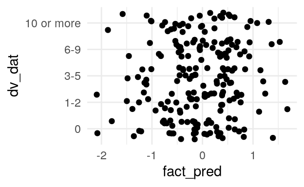
| lhs | op | rhs | est | se | z | pvalue | ci.lower | ci.upper | std.lv | std.all | std.nox |
|---|---|---|---|---|---|---|---|---|---|---|---|
| alcohol_days_of_lst30 | ~ | fsmi_stat | 0.06 | 0.10 | 0.59 | 0.56 | -0.14 | 0.25 | 0.05 | 0.05 | 0.05 |
| alcohol_days_of_lst30 | ~ | gender_c | -0.22 | 0.16 | -1.34 | 0.18 | -0.53 | 0.10 | -0.22 | -0.10 | -0.21 |
| lhs | op | rhs | est | se | z | pvalue | ci.lower | ci.upper | std.lv | std.all | std.nox |
|---|---|---|---|---|---|---|---|---|---|---|---|
| alcohol_days_of_lst30 | ~ | neg_urgency | -0.13 | 0.36 | -0.36 | 0.72 | -0.83 | 0.57 | -0.06 | -0.06 | -0.06 |
| alcohol_days_of_lst30 | ~ | sensation_seeking | 0.61 | 0.19 | 3.25 | 0.00 | 0.24 | 0.98 | 0.29 | 0.29 | 0.29 |
| alcohol_days_of_lst30 | ~ | pos_urgency | 0.13 | 0.28 | 0.46 | 0.64 | -0.41 | 0.67 | 0.08 | 0.08 | 0.08 |
| alcohol_days_of_lst30 | ~ | fsmi_stat | 0.00 | 0.00 | 0.00 | 0.00 | 0.00 | 0.00 | 0.00 | ||
| alcohol_days_of_lst30 | ~ | gender_c | -0.18 | 0.18 | -0.99 | 0.32 | -0.53 | 0.17 | -0.18 | -0.08 | -0.18 |
| lhs | op | rhs | est | se | z | pvalue | ci.lower | ci.upper | std.lv | std.all | std.nox |
|---|---|---|---|---|---|---|---|---|---|---|---|
| alcohol_days_of_lst30 | ~ | neg_urgency | -0.02 | 0.36 | -0.06 | 0.95 | -0.73 | 0.69 | -0.01 | -0.01 | -0.01 |
| alcohol_days_of_lst30 | ~ | sensation_seeking | 0.68 | 0.20 | 3.39 | 0.00 | 0.29 | 1.07 | 0.32 | 0.32 | 0.32 |
| alcohol_days_of_lst30 | ~ | pos_urgency | 0.06 | 0.27 | 0.24 | 0.81 | -0.47 | 0.60 | 0.04 | 0.04 | 0.04 |
| alcohol_days_of_lst30 | ~ | fsmi_stat | -0.07 | 0.10 | -0.72 | 0.47 | -0.28 | 0.13 | -0.07 | -0.07 | -0.07 |
| alcohol_days_of_lst30 | ~ | gender_c | -0.18 | 0.18 | -0.99 | 0.32 | -0.53 | 0.17 | -0.18 | -0.08 | -0.18 |
The following models test whether drinking behavior is associated with FSMI Status, or K-SRQ Admiration variables. As above, initial models include both the focal motive variable and gender, which are compared to models in which the coefficient for the motive variable is fixed to zero. Significant decrease in fit is taken as evidence for an association between the motive variable and the behavioral outcome.
In the next step, the initial model is augmented by adding UPPS-P Sensation Seeking, Positive Urgency, and Negative Urgency, with the same constraint of the focal motive variable tested. Significant difference in fit here indicates that the focal motive is associated with the outcome even when conditioning on (or perhaps because of this conditioning) the UPPS-P impulsivity and sensation-seeking variables.
For the K-SRQ, an additional test is made by including the Sociability variable in the regression. Significant decrease in fit when the coefficient for this variable is fixed to zero indicates that it has an association with the behavioral outcome over and above the variance it shares with the Admiration variable. The coefficients between the unconstrained and constrained model will also be examined.
K-SRQ Admiration
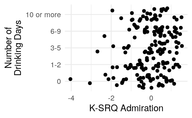
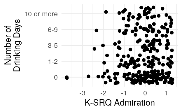
#> Scaled Chi Square Difference Test (method = "satorra.2000")
#>
#>                         Df AIC BIC   Chisq Chisq diff Df diff Pr(>Chisq)
#> ksrq_nosoc_alc_days_sem 84          90.931
#> ksrq_alc_days_null_sem  85         157.084     12.975       1  0.0003157 ***
#> ---
#> Signif. codes:  0 '***' 0.001 '**' 0.01 '*' 0.05 '.' 0.1 ' ' 1
#> Scaled Chi Square Difference Test (method = "satorra.2000")
#>
#>                             Df AIC BIC  Chisq Chisq diff Df diff Pr(>Chisq)
#> ksrq_nosoc_alc_days_all_sem 97         193.25
#> ksrq_alc_days_null_all_sem  98         261.15     15.262       1  9.359e-05 ***
#> ---
#> Signif. codes:  0 '***' 0.001 '**' 0.01 '*' 0.05 '.' 0.1 ' ' 1
#> Scaled Chi Square Difference Test (method = "satorra.2000")
#>
#>                         Df AIC BIC  Chisq Chisq diff Df diff Pr(>Chisq)
#> ksrq_alc_days_sem       83         76.456
#> ksrq_nosoc_alc_days_sem 84         90.931     12.566       1  0.0003928 ***
#> ---
#> Signif. codes:  0 '***' 0.001 '**' 0.01 '*' 0.05 '.' 0.1 ' ' 1
#> Scaled Chi Square Difference Test (method = "satorra.2000")
#>
#>                             Df AIC BIC  Chisq Chisq diff Df diff Pr(>Chisq)
#> ksrq_alc_days_all_sem       96         166.65
#> ksrq_nosoc_alc_days_all_sem 97         193.25       21.1       1  4.358e-06 ***
#> ---
#> Signif. codes:  0 '***' 0.001 '**' 0.01 '*' 0.05 '.' 0.1 ' ' 1
#> Scaled Chi Square Difference Test (method = "satorra.2000")
#>
#>                                Df AIC BIC  Chisq Chisq diff Df diff Pr(>Chisq)
#> uppsp_ksrq_alc_days_sem      1301         1786.2
#> uppsp_ksrq_nosr_alc_days_sem 1302         1792.5     2.4412       1     0.1182
#> Scaled Chi Square Difference Test (method = "satorra.2000")
#>
#>                                     Df AIC BIC  Chisq Chisq diff Df diff
#> uppsp_ksrq_alc_days_all__sem      1352         2263.9
#> uppsp_ksrq_nosr_alc_days_all__sem 1353         2268.1     1.6796       1
#>                                   Pr(>Chisq)
#> uppsp_ksrq_alc_days_all__sem
#> uppsp_ksrq_nosr_alc_days_all__sem 0.195| lhs | op | rhs | est | se | z | pvalue | ci.lower | ci.upper | std.lv | std.all | std.nox |
|---|---|---|---|---|---|---|---|---|---|---|---|
| alcohol_days_of_lst30 | ~ | k_srq_admiration | -0.55 | 0.21 | -2.57 | 0.01 | -0.97 | -0.13 | -0.55 | -0.55 | -0.55 |
| alcohol_days_of_lst30 | ~ | k_srq_sociability | 1.02 | 0.28 | 3.63 | 0.00 | 0.47 | 1.57 | 0.85 | 0.85 | 0.85 |
| alcohol_days_of_lst30 | ~ | gender_c | -0.13 | 0.17 | -0.80 | 0.42 | -0.46 | 0.19 | -0.13 | -0.06 | -0.13 |
| lhs | op | rhs | est | se | z | pvalue | ci.lower | ci.upper | std.lv | std.all | std.nox |
|---|---|---|---|---|---|---|---|---|---|---|---|
| alcohol_days_of_lst30 | ~ | k_srq_admiration | 0.30 | 0.08 | 4.01 | 0.00 | 0.15 | 0.45 | 0.30 | 0.30 | 0.30 |
| alcohol_days_of_lst30 | ~ | k_srq_sociability | 0.00 | 0.00 | 0.00 | 0.00 | 0.00 | 0.00 | 0.00 | ||
| alcohol_days_of_lst30 | ~ | gender_c | -0.13 | 0.17 | -0.80 | 0.42 | -0.46 | 0.19 | -0.13 | -0.06 | -0.13 |
| lhs | op | rhs | est | se | z | pvalue | ci.lower | ci.upper | std.lv | std.all | std.nox |
|---|---|---|---|---|---|---|---|---|---|---|---|
| alcohol_days_of_lst30 | ~ | k_srq_admiration | -0.28 | 0.13 | -2.20 | 0.03 | -0.54 | -0.03 | -0.27 | -0.21 | -0.21 |
| alcohol_days_of_lst30 | ~ | k_srq_sociability | 0.69 | 0.16 | 4.32 | 0.00 | 0.38 | 1.00 | 0.60 | 0.47 | 0.47 |
| alcohol_days_of_lst30 | ~ | gender_c | 0.16 | 0.15 | 1.04 | 0.30 | -0.14 | 0.45 | 0.16 | 0.06 | 0.12 |
| alcohol_days_of_lst30 | ~ | age_c | 0.34 | 0.04 | 9.12 | 0.00 | 0.27 | 0.42 | 0.34 | 0.61 | 0.27 |
| lhs | op | rhs | est | se | z | pvalue | ci.lower | ci.upper | std.lv | std.all | std.nox |
|---|---|---|---|---|---|---|---|---|---|---|---|
| alcohol_days_of_lst30 | ~ | k_srq_admiration | 0.31 | 0.07 | 4.26 | 0.0 | 0.17 | 0.45 | 0.28 | 0.22 | 0.22 |
| alcohol_days_of_lst30 | ~ | k_srq_sociability | 0.00 | 0.00 | 0.00 | 0.00 | 0.00 | 0.00 | 0.00 | ||
| alcohol_days_of_lst30 | ~ | gender_c | 0.16 | 0.15 | 1.04 | 0.3 | -0.14 | 0.45 | 0.16 | 0.06 | 0.12 |
| alcohol_days_of_lst30 | ~ | age_c | 0.34 | 0.04 | 9.12 | 0.0 | 0.27 | 0.42 | 0.34 | 0.61 | 0.27 |
| lhs | op | rhs | est | se | z | pvalue | ci.lower | ci.upper | std.lv | std.all | std.nox |
|---|---|---|---|---|---|---|---|---|---|---|---|
| alcohol_days_of_lst30 | ~ | neg_urgency | 0.01 | 0.37 | 0.02 | 0.98 | -0.72 | 0.74 | 0.00 | 0.00 | 0.00 |
| alcohol_days_of_lst30 | ~ | sensation_seeking | 0.70 | 0.19 | 3.65 | 0.00 | 0.32 | 1.07 | 0.34 | 0.34 | 0.34 |
| alcohol_days_of_lst30 | ~ | pos_urgency | -0.10 | 0.27 | -0.37 | 0.71 | -0.63 | 0.43 | -0.06 | -0.06 | -0.06 |
| alcohol_days_of_lst30 | ~ | k_srq_admiration | 0.17 | 0.10 | 1.75 | 0.08 | -0.02 | 0.35 | 0.16 | 0.16 | 0.16 |
| alcohol_days_of_lst30 | ~ | gender_c | -0.16 | 0.18 | -0.90 | 0.37 | -0.52 | 0.19 | -0.16 | -0.07 | -0.16 |
| lhs | op | rhs | est | se | z | pvalue | ci.lower | ci.upper | std.lv | std.all | std.nox |
|---|---|---|---|---|---|---|---|---|---|---|---|
| alcohol_days_of_lst30 | ~ | neg_urgency | 0.87 | 0.56 | 1.54 | 0.12 | -0.23 | 1.97 | 0.41 | 0.41 | 0.41 |
| alcohol_days_of_lst30 | ~ | sensation_seeking | 0.83 | 0.20 | 4.19 | 0.00 | 0.44 | 1.21 | 0.41 | 0.41 | 0.41 |
| alcohol_days_of_lst30 | ~ | pos_urgency | -0.74 | 0.44 | -1.69 | 0.09 | -1.60 | 0.12 | -0.47 | -0.47 | -0.47 |
| alcohol_days_of_lst30 | ~ | k_srq_admiration | 0.00 | 0.00 | 0.00 | 0.00 | 0.00 | 0.00 | 0.00 | ||
| alcohol_days_of_lst30 | ~ | gender_c | -0.16 | 0.18 | -0.90 | 0.37 | -0.52 | 0.19 | -0.16 | -0.07 | -0.16 |
| lhs | op | rhs | est | se | z | pvalue | ci.lower | ci.upper | std.lv | std.all | std.nox |
|---|---|---|---|---|---|---|---|---|---|---|---|
| alcohol_days_of_lst30 | ~ | neg_urgency | 0.15 | 0.33 | 0.46 | 0.64 | -0.50 | 0.80 | 0.08 | 0.06 | 0.06 |
| alcohol_days_of_lst30 | ~ | sensation_seeking | 0.66 | 0.18 | 3.74 | 0.00 | 0.31 | 1.00 | 0.32 | 0.25 | 0.25 |
| alcohol_days_of_lst30 | ~ | pos_urgency | -0.09 | 0.25 | -0.37 | 0.71 | -0.58 | 0.40 | -0.06 | -0.05 | -0.05 |
| alcohol_days_of_lst30 | ~ | k_srq_admiration | 0.14 | 0.09 | 1.50 | 0.13 | -0.04 | 0.33 | 0.13 | 0.10 | 0.10 |
| alcohol_days_of_lst30 | ~ | gender_c | 0.10 | 0.16 | 0.63 | 0.53 | -0.22 | 0.42 | 0.10 | 0.04 | 0.08 |
| alcohol_days_of_lst30 | ~ | age_c | 0.34 | 0.04 | 8.31 | 0.00 | 0.26 | 0.42 | 0.34 | 0.61 | 0.27 |
| lhs | op | rhs | est | se | z | pvalue | ci.lower | ci.upper | std.lv | std.all | std.nox |
|---|---|---|---|---|---|---|---|---|---|---|---|
| alcohol_days_of_lst30 | ~ | neg_urgency | 0.72 | 0.42 | 1.72 | 0.09 | -0.10 | 1.54 | 0.36 | 0.28 | 0.28 |
| alcohol_days_of_lst30 | ~ | sensation_seeking | 0.78 | 0.18 | 4.41 | 0.00 | 0.43 | 1.13 | 0.38 | 0.30 | 0.30 |
| alcohol_days_of_lst30 | ~ | pos_urgency | -0.53 | 0.32 | -1.64 | 0.10 | -1.17 | 0.10 | -0.35 | -0.28 | -0.28 |
| alcohol_days_of_lst30 | ~ | k_srq_admiration | 0.00 | 0.00 | 0.00 | 0.00 | 0.00 | 0.00 | 0.00 | ||
| alcohol_days_of_lst30 | ~ | gender_c | 0.10 | 0.16 | 0.63 | 0.53 | -0.22 | 0.42 | 0.10 | 0.04 | 0.08 |
| alcohol_days_of_lst30 | ~ | age_c | 0.34 | 0.04 | 8.31 | 0.00 | 0.26 | 0.42 | 0.34 | 0.61 | 0.27 |
K-SRQ Admiration is positively associated with number drinking days when considering the both the college and full sample. Controlling for levels of K-SRQ Sociability results in a reversal of the sign of the coefficient and an increase in magnitude. Removing the Sociability scale from this model does significantly decrease fit. The sign of the Sociability coeficient is positive. Together, this indicating that for a given level of Sociability, higher levels on Admiration are negatively associated with number of drinking days. Comparing a model with Admiration, and UPPS-P Sensation Seeking and (+/-) Urgency, to the same model with the coefficient for Admiration fixed to zero does not result in a significant reduction of fit. The coefficients for both Sensation Seeking and Admiration in the combine model are positive.
SPLT parameters
#> Scaled Chi Square Difference Test (method = "satorra.2000")
#>
#>                        Df AIC BIC  Chisq Chisq diff Df diff Pr(>Chisq)
#> splt_alc_days_sem       9         3.9743
#> splt_alc_days_null_sem 10         7.4320     1.1939       1     0.2745
#> Scaled Chi Square Difference Test (method = "satorra.2000")
#>
#>                            Df AIC BIC  Chisq Chisq diff Df diff Pr(>Chisq)
#> splt_alc_days_all_sem      14         19.799
#> splt_alc_days_all_null_sem 15         20.018   0.074902       1     0.7843
#> Scaled Chi Square Difference Test (method = "satorra.2000")
#>
#>                        Df AIC BIC  Chisq Chisq diff Df diff Pr(>Chisq)
#> splt_alc_days_sem       9         10.349
#> splt_alc_days_null_sem 10         13.174    0.67597       1      0.411
#> Scaled Chi Square Difference Test (method = "satorra.2000")
#>
#>                            Df AIC BIC  Chisq Chisq diff Df diff Pr(>Chisq)
#> splt_alc_days_all_sem      14         6.6693
#> splt_alc_days_all_null_sem 15         8.2557    0.37472       1     0.5404
#> Scaled Chi Square Difference Test (method = "satorra.2000")
#>
#>                        Df AIC BIC  Chisq Chisq diff Df diff Pr(>Chisq)
#> splt_alc_days_sem       9         34.923
#> splt_alc_days_null_sem 10         35.214    0.17799       1     0.6731
#> Scaled Chi Square Difference Test (method = "satorra.2000")
#>
#>                            Df AIC BIC  Chisq Chisq diff Df diff Pr(>Chisq)
#> splt_alc_days_all_sem      14         23.706
#> splt_alc_days_all_null_sem 15         27.948     2.8026       1    0.09411 .
#> ---
#> Signif. codes:  0 '***' 0.001 '**' 0.01 '*' 0.05 '.' 0.1 ' ' 1
#> Scaled Chi Square Difference Test (method = "satorra.2000")
#>
#>                        Df AIC BIC  Chisq Chisq diff Df diff Pr(>Chisq)
#> splt_alc_days_sem       9         0.3764
#> splt_alc_days_null_sem 10         1.3005    0.45962       1     0.4978
#> Scaled Chi Square Difference Test (method = "satorra.2000")
#>
#>                            Df AIC BIC  Chisq Chisq diff Df diff Pr(>Chisq)
#> splt_alc_days_all_sem      14         7.0302
#> splt_alc_days_all_null_sem 15         8.6065    0.74398       1     0.3884
#> Scaled Chi Square Difference Test (method = "satorra.2000")
#>
#>                        Df AIC BIC  Chisq Chisq diff Df diff Pr(>Chisq)
#> splt_alc_days_sem       9         7.3702
#> splt_alc_days_null_sem 10         7.9343     0.2748       1     0.6001
#> Scaled Chi Square Difference Test (method = "satorra.2000")
#>
#>                            Df AIC BIC  Chisq Chisq diff Df diff Pr(>Chisq)
#> splt_alc_days_all_sem      14         19.521
#> splt_alc_days_all_null_sem 15         21.836     1.1588       1     0.2817
#> Scaled Chi Square Difference Test (method = "satorra.2000")
#>
#>                        Df AIC BIC  Chisq Chisq diff Df diff Pr(>Chisq)
#> splt_alc_days_sem       9         12.403
#> splt_alc_days_null_sem 10         13.501    0.66094       1     0.4162
#> Scaled Chi Square Difference Test (method = "satorra.2000")
#>
#>                            Df AIC BIC  Chisq Chisq diff Df diff Pr(>Chisq)
#> splt_alc_days_all_sem      14         14.421
#> splt_alc_days_all_null_sem 15         14.695    0.16241       1     0.6869
#>
#>
#> Table: (\#tab:unnamed-chunk-69)$\epsilon$ predicting number of drinking dats among college students; N obs. = 212
#>
#> lhs                     op   rhs                       est     se       z   pvalue   ci.lower   ci.upper   std.lv   std.all   std.nox
#> ----------------------  ---  ---------------------  ------  -----  ------  -------  ---------  ---------  -------  --------  --------
#> alcohol_days_of_lst30   ~    ep_prm_PplrUHngT_fac    -1.39   1.26   -1.11     0.27      -3.86       1.07    -0.09     -0.09     -0.09
#> alcohol_days_of_lst30   ~    gender_c                -0.22   0.16   -1.39     0.16      -0.53       0.09    -0.22     -0.10     -0.22
#>
#>
#> Table: (\#tab:unnamed-chunk-69)$\epsilon$ predicting number of drinking dats among all adolescent and college participants with SES responses; N obs. = 298
#>
#> lhs                     op   rhs                       est     se       z   pvalue   ci.lower   ci.upper   std.lv   std.all   std.nox
#> ----------------------  ---  ---------------------  ------  -----  ------  -------  ---------  ---------  -------  --------  --------
#> alcohol_days_of_lst30   ~    ep_prm_PplrUHngT_fac    -0.34   1.24   -0.27     0.78      -2.78       2.09    -0.02     -0.02     -0.02
#> alcohol_days_of_lst30   ~    gender_c                 0.08   0.14    0.54     0.59      -0.20       0.36     0.08      0.03      0.06
#> alcohol_days_of_lst30   ~    age_c                    0.32   0.04    8.62     0.00       0.25       0.39     0.32      0.58      0.26
#>
#>
#> Table: (\#tab:unnamed-chunk-69)$\rho$ predicting number of drinking dats among college students; N obs. = 212
#>
#> lhs                     op   rhs                        est     se       z   pvalue   ci.lower   ci.upper   std.lv   std.all   std.nox
#> ----------------------  ---  ----------------------  ------  -----  ------  -------  ---------  ---------  -------  --------  --------
#> alcohol_days_of_lst30   ~    rho_prm_PplrUHngT_fac    -0.09   0.11   -0.83     0.41      -0.30       0.12    -0.06     -0.06     -0.06
#> alcohol_days_of_lst30   ~    gender_c                 -0.22   0.16   -1.39     0.16      -0.53       0.09    -0.22     -0.10     -0.22
#>
#>
#> Table: (\#tab:unnamed-chunk-69)$\rho$ predicting number of drinking dats among all adolescent and college participants with SES responses; N obs. = 298
#>
#> lhs                     op   rhs                        est     se       z   pvalue   ci.lower   ci.upper   std.lv   std.all   std.nox
#> ----------------------  ---  ----------------------  ------  -----  ------  -------  ---------  ---------  -------  --------  --------
#> alcohol_days_of_lst30   ~    rho_prm_PplrUHngT_fac    -0.06   0.10   -0.61     0.54      -0.26       0.14    -0.04     -0.03     -0.03
#> alcohol_days_of_lst30   ~    gender_c                  0.08   0.14    0.54     0.59      -0.20       0.36     0.08      0.03      0.06
#> alcohol_days_of_lst30   ~    age_c                     0.32   0.04    8.62     0.00       0.25       0.39     0.32      0.58      0.26
#>
#>
#> Table: (\#tab:unnamed-chunk-69)$\xi$ predicting number of drinking dats among college students; N obs. = 212
#>
#> lhs                     op   rhs                       est     se       z   pvalue   ci.lower   ci.upper   std.lv   std.all   std.nox
#> ----------------------  ---  ---------------------  ------  -----  ------  -------  ---------  ---------  -------  --------  --------
#> alcohol_days_of_lst30   ~    xi_prm_PplrUHngT_fac     0.37   0.85    0.44     0.66      -1.29       2.03     0.03      0.03      0.03
#> alcohol_days_of_lst30   ~    gender_c                -0.22   0.16   -1.39     0.16      -0.53       0.09    -0.22     -0.10     -0.22
#>
#>
#> Table: (\#tab:unnamed-chunk-69)$\xi$ predicting number of drinking dats among all adolescent and college participants with SES responses; N obs. = 298
#>
#> lhs                     op   rhs                      est     se      z   pvalue   ci.lower   ci.upper   std.lv   std.all   std.nox
#> ----------------------  ---  ---------------------  -----  -----  -----  -------  ---------  ---------  -------  --------  --------
#> alcohol_days_of_lst30   ~    xi_prm_PplrUHngT_fac    1.15   0.71   1.62     0.11      -0.24       2.54     0.10      0.08      0.08
#> alcohol_days_of_lst30   ~    gender_c                0.08   0.14   0.54     0.59      -0.20       0.36     0.08      0.03      0.06
#> alcohol_days_of_lst30   ~    age_c                   0.32   0.04   8.62     0.00       0.25       0.39     0.32      0.58      0.26
#>
#>
#> Table: (\#tab:unnamed-chunk-69)$b$ predicting number of drinking dats among college students; N obs. = 212
#>
#> lhs                     op   rhs                  est     se       z   pvalue   ci.lower   ci.upper   std.lv   std.all   std.nox
#> ----------------------  ---  ----------------  ------  -----  ------  -------  ---------  ---------  -------  --------  --------
#> alcohol_days_of_lst30   ~    b_PplrUHngT_fac     0.17   0.26    0.68     0.50      -0.33       0.68     0.05      0.05      0.05
#> alcohol_days_of_lst30   ~    gender_c           -0.22   0.16   -1.39     0.16      -0.53       0.09    -0.22     -0.10     -0.22
#>
#>
#> Table: (\#tab:unnamed-chunk-69)$b$ predicting number of drinking dats among all adolescent and college participants with SES responses; N obs. = 298
#>
#> lhs                     op   rhs                 est     se      z   pvalue   ci.lower   ci.upper   std.lv   std.all   std.nox
#> ----------------------  ---  ----------------  -----  -----  -----  -------  ---------  ---------  -------  --------  --------
#> alcohol_days_of_lst30   ~    b_PplrUHngT_fac    0.21   0.24   0.86     0.39      -0.27       0.69     0.06      0.05      0.05
#> alcohol_days_of_lst30   ~    gender_c           0.08   0.14   0.54     0.59      -0.20       0.36     0.08      0.03      0.06
#> alcohol_days_of_lst30   ~    age_c              0.32   0.04   8.62     0.00       0.25       0.39     0.32      0.58      0.26
#>
#>
#> Table: (\#tab:unnamed-chunk-69)First-half optimal responses predicting number of drinking dats among college students; N obs. = 212
#>
#> lhs                     op   rhs                               est     se       z   pvalue   ci.lower   ci.upper   std.lv   std.all   std.nox
#> ----------------------  ---  -----------------------------  ------  -----  ------  -------  ---------  ---------  -------  --------  --------
#> alcohol_days_of_lst30   ~    bin_start_to_4_PplrUHngT_fac    -0.25   0.47   -0.52     0.60      -1.18       0.68    -0.04     -0.04     -0.04
#> alcohol_days_of_lst30   ~    gender_c                        -0.22   0.16   -1.39     0.16      -0.53       0.09    -0.22     -0.10     -0.22
#>
#>
#> Table: (\#tab:unnamed-chunk-69)First-half optimal responses predicting number of drinking dats among all adolescent and college participants with SES responses; N obs. = 298
#>
#> lhs                     op   rhs                               est     se       z   pvalue   ci.lower   ci.upper   std.lv   std.all   std.nox
#> ----------------------  ---  -----------------------------  ------  -----  ------  -------  ---------  ---------  -------  --------  --------
#> alcohol_days_of_lst30   ~    bin_start_to_4_PplrUHngT_fac    -0.44   0.41   -1.08     0.28      -1.24       0.36    -0.06     -0.05     -0.05
#> alcohol_days_of_lst30   ~    gender_c                         0.08   0.14    0.54     0.59      -0.20       0.36     0.08      0.03      0.06
#> alcohol_days_of_lst30   ~    age_c                            0.32   0.04    8.62     0.00       0.25       0.39     0.32      0.58      0.26
#>
#>
#> Table: (\#tab:unnamed-chunk-69)Last-half optimal responses predicting number of drinking dats among college students; N obs. = 212
#>
#> lhs                     op   rhs                             est     se       z   pvalue   ci.lower   ci.upper   std.lv   std.all   std.nox
#> ----------------------  ---  ---------------------------  ------  -----  ------  -------  ---------  ---------  -------  --------  --------
#> alcohol_days_of_lst30   ~    bin_5_to_end_PplrUHngT_fac     0.47   0.57    0.82     0.41      -0.65       1.58     0.06      0.06      0.06
#> alcohol_days_of_lst30   ~    gender_c                      -0.22   0.16   -1.39     0.16      -0.53       0.09    -0.22     -0.10     -0.22
#>
#>
#> Table: (\#tab:unnamed-chunk-69)Last-half optimal responses predicting number of drinking dats among all adolescent and college participants with SES responses; N obs. = 298
#>
#> lhs                     op   rhs                             est     se       z   pvalue   ci.lower   ci.upper   std.lv   std.all   std.nox
#> ----------------------  ---  ---------------------------  ------  -----  ------  -------  ---------  ---------  -------  --------  --------
#> alcohol_days_of_lst30   ~    bin_5_to_end_PplrUHngT_fac    -0.20   0.49   -0.40     0.69      -1.16       0.77    -0.03     -0.02     -0.02
#> alcohol_days_of_lst30   ~    gender_c                       0.08   0.14    0.54     0.59      -0.20       0.36     0.08      0.03      0.06
#> alcohol_days_of_lst30   ~    age_c                          0.32   0.04    8.62     0.00       0.25       0.39     0.32      0.58      0.26
Again, no \(\chi^2\) tests satisfy the \(\alpha = .005\) cutoff.
Number of days during which 5+ alcoholic drinks were consumed
FSMI Status
#> Scaled Chi Square Difference Test (method = "satorra.2000")
#>
#>                         Df AIC BIC   Chisq Chisq diff Df diff Pr(>Chisq)
#> fsmi_alc_5drnk_sem      76          96.313
#> fsmi_alc_5drnk_null_sem 77         100.560     1.8339       1     0.1757
#> Scaled Chi Square Difference Test (method = "satorra.2000")
#>
#>                                Df AIC BIC  Chisq Chisq diff Df diff Pr(>Chisq)
#> uppsp_fsmi_alc5drk_sem        980         1543.4
#> uppsp_fsmi_alc5drk_noupps_sem 983         1603.8     10.284   2.007  0.0058958
#> uppsp_fsmi_alc5drk_null_sem   984         1689.3     13.485   1.000  0.0002405
#>
#> uppsp_fsmi_alc5drk_sem
#> uppsp_fsmi_alc5drk_noupps_sem **
#> uppsp_fsmi_alc5drk_null_sem   ***
#> ---
#> Signif. codes:  0 '***' 0.001 '**' 0.01 '*' 0.05 '.' 0.1 ' ' 1
#> Scaled Chi Square Difference Test (method = "satorra.2000")
#>
#>                                Df AIC BIC  Chisq Chisq diff Df diff Pr(>Chisq)
#> uppsp_fsmi_alc5drk_sem        980         1543.4
#> uppsp_fsmi_alc5drk_nofsmi_sem 981         1543.5     0.0072   1.000  0.9325527
#> uppsp_fsmi_alc5drk_null_sem   984         1689.3    16.9337   1.933  0.0001912
#>
#> uppsp_fsmi_alc5drk_sem
#> uppsp_fsmi_alc5drk_nofsmi_sem
#> uppsp_fsmi_alc5drk_null_sem   ***
#> ---
#> Signif. codes:  0 '***' 0.001 '**' 0.01 '*' 0.05 '.' 0.1 ' ' 1
#> Scaled Chi Square Difference Test (method = "satorra.2000")
#>
#>                                Df AIC BIC  Chisq Chisq diff Df diff Pr(>Chisq)
#> uppsp_fsmi_alc5drk_sem        980         1543.4
#> uppsp_fsmi_alc5drk_nopurg_sem 981         1543.5     0.0557   1.000  0.8135061
#> uppsp_fsmi_alc5drk_null_sem   984         1689.3    17.1931   1.982  0.0001801
#>
#> uppsp_fsmi_alc5drk_sem
#> uppsp_fsmi_alc5drk_nopurg_sem
#> uppsp_fsmi_alc5drk_null_sem   ***
#> ---
#> Signif. codes:  0 '***' 0.001 '**' 0.01 '*' 0.05 '.' 0.1 ' ' 1
#> Scaled Chi Square Difference Test (method = "satorra.2000")
#>
#>                                Df AIC BIC  Chisq Chisq diff Df diff Pr(>Chisq)
#> uppsp_fsmi_alc5drk_sem        980         1543.4
#> uppsp_fsmi_alc5drk_nonurg_sem 981         1544.6     0.8906  1.0000  0.3453108
#> uppsp_fsmi_alc5drk_null_sem   984         1689.3    16.9987  1.9888  0.0002004
#>
#> uppsp_fsmi_alc5drk_sem
#> uppsp_fsmi_alc5drk_nonurg_sem
#> uppsp_fsmi_alc5drk_null_sem   ***
#> ---
#> Signif. codes:  0 '***' 0.001 '**' 0.01 '*' 0.05 '.' 0.1 ' ' 1
#> Scaled Chi Square Difference Test (method = "satorra.2000")
#>
#>                              Df AIC BIC  Chisq Chisq diff Df diff Pr(>Chisq)
#> uppsp_fsmi_alc5drk_sem      980         1543.4
#> uppsp_fsmi_alc5drk_noss_sem 981         1568.2      9.821  1.0000  0.0017253
#> uppsp_fsmi_alc5drk_null_sem 984         1689.3     14.034  1.8404  0.0007216
#>
#> uppsp_fsmi_alc5drk_sem
#> uppsp_fsmi_alc5drk_noss_sem **
#> uppsp_fsmi_alc5drk_null_sem ***
#> ---
#> Signif. codes:  0 '***' 0.001 '**' 0.01 '*' 0.05 '.' 0.1 ' ' 1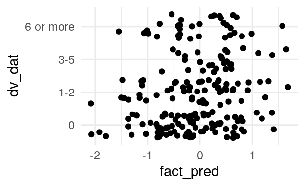
| lhs | op | rhs | est.std | se | z | pvalue | ci.lower | ci.upper |
|---|---|---|---|---|---|---|---|---|
| alcohol_5drnks_lst30 | ~ | fsmi_stat | 0.12 | 0.09 | 1.39 | 0.16 | -0.05 | 0.30 |
| alcohol_5drnks_lst30 | ~ | gender_c | -0.17 | 0.07 | -2.29 | 0.02 | -0.32 | -0.02 |
| lhs | op | rhs | est.std | se | z | pvalue | ci.lower | ci.upper |
|---|---|---|---|---|---|---|---|---|
| alcohol_5drnks_lst30 | ~ | neg_urgency | 0.20 | 0.22 | 0.90 | 0.37 | -0.23 | 0.63 |
| alcohol_5drnks_lst30 | ~ | sensation_seeking | 0.31 | 0.09 | 3.57 | 0.00 | 0.14 | 0.48 |
| alcohol_5drnks_lst30 | ~ | pos_urgency | -0.04 | 0.22 | -0.20 | 0.84 | -0.48 | 0.39 |
| alcohol_5drnks_lst30 | ~ | fsmi_stat | 0.00 | 0.00 | 0.00 | 0.00 | ||
| alcohol_5drnks_lst30 | ~ | gender_c | -0.15 | 0.08 | -1.77 | 0.08 | -0.31 | 0.02 |
| lhs | op | rhs | est.std | se | z | pvalue | ci.lower | ci.upper |
|---|---|---|---|---|---|---|---|---|
| alcohol_5drnks_lst30 | ~ | neg_urgency | 0.21 | 0.21 | 0.96 | 0.34 | -0.22 | 0.63 |
| alcohol_5drnks_lst30 | ~ | sensation_seeking | 0.31 | 0.09 | 3.51 | 0.00 | 0.14 | 0.49 |
| alcohol_5drnks_lst30 | ~ | pos_urgency | -0.05 | 0.21 | -0.24 | 0.81 | -0.46 | 0.36 |
| alcohol_5drnks_lst30 | ~ | fsmi_stat | -0.01 | 0.10 | -0.09 | 0.93 | -0.20 | 0.19 |
| alcohol_5drnks_lst30 | ~ | gender_c | -0.15 | 0.08 | -1.77 | 0.08 | -0.31 | 0.02 |
In the college student sample, model fit does not decrease significantly when the association between number of heavy drinking days and FSMI Status is fixed to 0 for any model. However, as above, comparing the model that includes FSMI Status along with UPPS-P Sensation Seeking, and Negative and Positive Urgency to the same model with the coefficient for Sensation Seeking fixed to 0 shows significant fit decrease.
K-SRQ Admiration
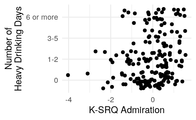
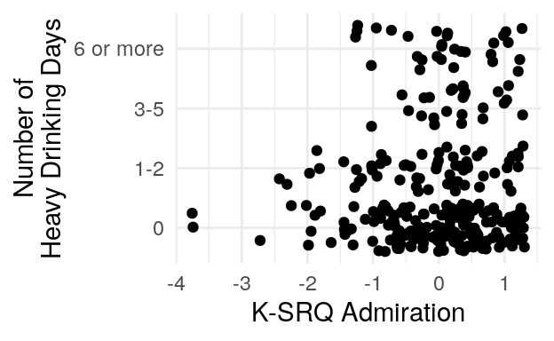
#> Scaled Chi Square Difference Test (method = "satorra.2000")
#>
#>                          Df AIC BIC   Chisq Chisq diff Df diff Pr(>Chisq)
#> ksrq_nosoc_alc_5drnk_sem 84          80.657
#> ksrq_alc_5drnk_null_sem  85         150.290      15.03       1  0.0001058 ***
#> ---
#> Signif. codes:  0 '***' 0.001 '**' 0.01 '*' 0.05 '.' 0.1 ' ' 1
#> Scaled Chi Square Difference Test (method = "satorra.2000")
#>
#>                              Df AIC BIC  Chisq Chisq diff Df diff Pr(>Chisq)
#> ksrq_nosoc_alc_5drnk_all_sem 97         193.52
#> ksrq_alc_5drnk_null_all_sem  98         265.96     16.446       1  5.005e-05
#>
#> ksrq_nosoc_alc_5drnk_all_sem
#> ksrq_alc_5drnk_null_all_sem  ***
#> ---
#> Signif. codes:  0 '***' 0.001 '**' 0.01 '*' 0.05 '.' 0.1 ' ' 1
#> Scaled Chi Square Difference Test (method = "satorra.2000")
#>
#>                          Df AIC BIC  Chisq Chisq diff Df diff Pr(>Chisq)
#> ksrq_alc_5drnk_sem       83         71.101
#> ksrq_nosoc_alc_5drnk_sem 84         80.657     8.2312       1   0.004118 **
#> ---
#> Signif. codes:  0 '***' 0.001 '**' 0.01 '*' 0.05 '.' 0.1 ' ' 1
#> Scaled Chi Square Difference Test (method = "satorra.2000")
#>
#>                              Df AIC BIC  Chisq Chisq diff Df diff Pr(>Chisq)
#> ksrq_alc_5drnk_all_sem       96         164.31
#> ksrq_nosoc_alc_5drnk_all_sem 97         193.52     20.601       1  5.657e-06
#>
#> ksrq_alc_5drnk_all_sem
#> ksrq_nosoc_alc_5drnk_all_sem ***
#> ---
#> Signif. codes:  0 '***' 0.001 '**' 0.01 '*' 0.05 '.' 0.1 ' ' 1
#> Scaled Chi Square Difference Test (method = "satorra.2000")
#>
#>                                 Df AIC BIC  Chisq Chisq diff Df diff Pr(>Chisq)
#> uppsp_ksrq_alc_5drnk_sem      1301         1774.4
#> uppsp_ksrq_nosr_alc_5drnk_sem 1302         1781.1     2.4432       1      0.118
#> Scaled Chi Square Difference Test (method = "satorra.2000")
#>
#>                                      Df AIC BIC  Chisq Chisq diff Df diff
#> uppsp_ksrq_alc_5drnk_all__sem      1352         2263.0
#> uppsp_ksrq_nosr_alc_5drnk_all__sem 1353         2267.5     1.7526       1
#>                                    Pr(>Chisq)
#> uppsp_ksrq_alc_5drnk_all__sem
#> uppsp_ksrq_nosr_alc_5drnk_all__sem 0.1856| lhs | op | rhs | est | se | z | pvalue | ci.lower | ci.upper | std.lv | std.all | std.nox |
|---|---|---|---|---|---|---|---|---|---|---|---|
| alcohol_5drnks_lst30 | ~ | k_srq_admiration | -0.22 | 0.17 | -1.28 | 0.2 | -0.55 | 0.12 | -0.22 | -0.22 | -0.22 |
| alcohol_5drnks_lst30 | ~ | k_srq_sociability | 0.68 | 0.21 | 3.22 | 0.0 | 0.26 | 1.09 | 0.59 | 0.58 | 0.58 |
| alcohol_5drnks_lst30 | ~ | gender_c | -0.29 | 0.18 | -1.62 | 0.1 | -0.63 | 0.06 | -0.29 | -0.13 | -0.28 |
| lhs | op | rhs | est | se | z | pvalue | ci.lower | ci.upper | std.lv | std.all | std.nox |
|---|---|---|---|---|---|---|---|---|---|---|---|
| alcohol_5drnks_lst30 | ~ | k_srq_admiration | 0.35 | 0.08 | 4.40 | 0.0 | 0.19 | 0.50 | 0.34 | 0.34 | 0.34 |
| alcohol_5drnks_lst30 | ~ | k_srq_sociability | 0.00 | 0.00 | 0.00 | 0.00 | 0.00 | 0.00 | 0.00 | ||
| alcohol_5drnks_lst30 | ~ | gender_c | -0.29 | 0.18 | -1.62 | 0.1 | -0.63 | 0.06 | -0.29 | -0.13 | -0.28 |
| lhs | op | rhs | est | se | z | pvalue | ci.lower | ci.upper | std.lv | std.all | std.nox |
|---|---|---|---|---|---|---|---|---|---|---|---|
| alcohol_5drnks_lst30 | ~ | k_srq_admiration | -0.30 | 0.14 | -2.12 | 0.03 | -0.58 | -0.02 | -0.29 | -0.25 | -0.25 |
| alcohol_5drnks_lst30 | ~ | k_srq_sociability | 0.77 | 0.17 | 4.53 | 0.00 | 0.44 | 1.10 | 0.68 | 0.60 | 0.60 |
| alcohol_5drnks_lst30 | ~ | gender_c | -0.06 | 0.16 | -0.41 | 0.68 | -0.37 | 0.24 | -0.06 | -0.03 | -0.06 |
| alcohol_5drnks_lst30 | ~ | age_c | 0.23 | 0.04 | 5.47 | 0.00 | 0.15 | 0.31 | 0.23 | 0.47 | 0.20 |
| lhs | op | rhs | est | se | z | pvalue | ci.lower | ci.upper | std.lv | std.all | std.nox |
|---|---|---|---|---|---|---|---|---|---|---|---|
| alcohol_5drnks_lst30 | ~ | k_srq_admiration | 0.36 | 0.08 | 4.39 | 0.00 | 0.20 | 0.53 | 0.34 | 0.30 | 0.30 |
| alcohol_5drnks_lst30 | ~ | k_srq_sociability | 0.00 | 0.00 | 0.00 | 0.00 | 0.00 | 0.00 | 0.00 | ||
| alcohol_5drnks_lst30 | ~ | gender_c | -0.06 | 0.16 | -0.41 | 0.68 | -0.37 | 0.24 | -0.06 | -0.03 | -0.06 |
| alcohol_5drnks_lst30 | ~ | age_c | 0.23 | 0.04 | 5.47 | 0.00 | 0.15 | 0.31 | 0.23 | 0.47 | 0.20 |
| lhs | op | rhs | est | se | z | pvalue | ci.lower | ci.upper | std.lv | std.all | std.nox |
|---|---|---|---|---|---|---|---|---|---|---|---|
| alcohol_5drnks_lst30 | ~ | neg_urgency | 0.24 | 0.48 | 0.50 | 0.62 | -0.70 | 1.18 | 0.11 | 0.11 | 0.11 |
| alcohol_5drnks_lst30 | ~ | sensation_seeking | 0.59 | 0.20 | 3.02 | 0.00 | 0.21 | 0.98 | 0.29 | 0.29 | 0.29 |
| alcohol_5drnks_lst30 | ~ | pos_urgency | -0.02 | 0.34 | -0.07 | 0.95 | -0.69 | 0.64 | -0.01 | -0.01 | -0.01 |
| alcohol_5drnks_lst30 | ~ | k_srq_admiration | 0.20 | 0.10 | 1.90 | 0.06 | -0.01 | 0.40 | 0.19 | 0.19 | 0.19 |
| alcohol_5drnks_lst30 | ~ | gender_c | -0.28 | 0.19 | -1.46 | 0.14 | -0.64 | 0.09 | -0.28 | -0.13 | -0.27 |
| lhs | op | rhs | est | se | z | pvalue | ci.lower | ci.upper | std.lv | std.all | std.nox |
|---|---|---|---|---|---|---|---|---|---|---|---|
| alcohol_5drnks_lst30 | ~ | neg_urgency | 1.24 | 0.65 | 1.92 | 0.05 | -0.03 | 2.51 | 0.57 | 0.57 | 0.57 |
| alcohol_5drnks_lst30 | ~ | sensation_seeking | 0.75 | 0.20 | 3.74 | 0.00 | 0.36 | 1.14 | 0.37 | 0.37 | 0.37 |
| alcohol_5drnks_lst30 | ~ | pos_urgency | -0.76 | 0.47 | -1.61 | 0.11 | -1.69 | 0.17 | -0.48 | -0.48 | -0.48 |
| alcohol_5drnks_lst30 | ~ | k_srq_admiration | 0.00 | 0.00 | 0.00 | 0.00 | 0.00 | 0.00 | 0.00 | ||
| alcohol_5drnks_lst30 | ~ | gender_c | -0.28 | 0.19 | -1.46 | 0.14 | -0.64 | 0.09 | -0.28 | -0.13 | -0.27 |
| lhs | op | rhs | est | se | z | pvalue | ci.lower | ci.upper | std.lv | std.all | std.nox |
|---|---|---|---|---|---|---|---|---|---|---|---|
| alcohol_5drnks_lst30 | ~ | neg_urgency | 0.39 | 0.44 | 0.90 | 0.37 | -0.46 | 1.24 | 0.19 | 0.17 | 0.17 |
| alcohol_5drnks_lst30 | ~ | sensation_seeking | 0.55 | 0.19 | 2.86 | 0.00 | 0.17 | 0.93 | 0.27 | 0.24 | 0.24 |
| alcohol_5drnks_lst30 | ~ | pos_urgency | -0.10 | 0.32 | -0.31 | 0.75 | -0.73 | 0.53 | -0.07 | -0.06 | -0.06 |
| alcohol_5drnks_lst30 | ~ | k_srq_admiration | 0.17 | 0.11 | 1.58 | 0.11 | -0.04 | 0.38 | 0.15 | 0.14 | 0.14 |
| alcohol_5drnks_lst30 | ~ | gender_c | -0.07 | 0.17 | -0.41 | 0.68 | -0.40 | 0.26 | -0.07 | -0.03 | -0.06 |
| alcohol_5drnks_lst30 | ~ | age_c | 0.22 | 0.04 | 5.05 | 0.00 | 0.13 | 0.31 | 0.22 | 0.45 | 0.20 |
| lhs | op | rhs | est | se | z | pvalue | ci.lower | ci.upper | std.lv | std.all | std.nox |
|---|---|---|---|---|---|---|---|---|---|---|---|
| alcohol_5drnks_lst30 | ~ | neg_urgency | 1.09 | 0.52 | 2.09 | 0.04 | 0.07 | 2.12 | 0.53 | 0.47 | 0.47 |
| alcohol_5drnks_lst30 | ~ | sensation_seeking | 0.70 | 0.19 | 3.74 | 0.00 | 0.33 | 1.07 | 0.34 | 0.31 | 0.31 |
| alcohol_5drnks_lst30 | ~ | pos_urgency | -0.64 | 0.39 | -1.65 | 0.10 | -1.40 | 0.12 | -0.42 | -0.38 | -0.38 |
| alcohol_5drnks_lst30 | ~ | k_srq_admiration | 0.00 | 0.00 | 0.00 | 0.00 | 0.00 | 0.00 | 0.00 | ||
| alcohol_5drnks_lst30 | ~ | gender_c | -0.07 | 0.17 | -0.41 | 0.68 | -0.40 | 0.26 | -0.07 | -0.03 | -0.06 |
| alcohol_5drnks_lst30 | ~ | age_c | 0.22 | 0.04 | 5.05 | 0.00 | 0.13 | 0.31 | 0.22 | 0.45 | 0.20 |
K-SRQ Admiration is positively associated with number heavy drinking days when considering the both the college and full sample. Controlling for levels of K-SRQ Sociability results in a reversal of the sign of the coefficient. Removing the Sociability scale from this model does significantly decrease fit. The sign of the Sociability coeficient is positive in the model with both K-SRQ scales. Together, this indicates that for a given level of Sociability, higher levels on Admiration are negatively associated with more heavy-drinking days. Comparing a model with Admiration, and UPPS-P Sensation Seeking and (+/-) Urgency, to the same model with the coefficient for Admiration fixed to zero does not result in a significant reduction of fit. The coefficients for both Sensation Seeking and Admiration in the combined model are positive.
SPLT parameters
#> Scaled Chi Square Difference Test (method = "satorra.2000")
#>
#>                         Df AIC BIC   Chisq Chisq diff Df diff Pr(>Chisq)
#> splt_alc_5drnk_sem       9          6.0765
#> splt_alc_5drnk_null_sem 10         24.7818     6.3568       1    0.01169 *
#> ---
#> Signif. codes:  0 '***' 0.001 '**' 0.01 '*' 0.05 '.' 0.1 ' ' 1
#> Scaled Chi Square Difference Test (method = "satorra.2000")
#>
#>                             Df AIC BIC  Chisq Chisq diff Df diff Pr(>Chisq)
#> splt_alc_5drnk_all_sem      14         21.587
#> splt_alc_5drnk_all_null_sem 15         29.790     2.7767       1    0.09564 .
#> ---
#> Signif. codes:  0 '***' 0.001 '**' 0.01 '*' 0.05 '.' 0.1 ' ' 1
#> Scaled Chi Square Difference Test (method = "satorra.2000")
#>
#>                         Df AIC BIC  Chisq Chisq diff Df diff Pr(>Chisq)
#> splt_alc_5drnk_sem       9         10.945
#> splt_alc_5drnk_null_sem 10         10.991   0.011121       1      0.916
#> Scaled Chi Square Difference Test (method = "satorra.2000")
#>
#>                             Df AIC BIC  Chisq Chisq diff Df diff Pr(>Chisq)
#> splt_alc_5drnk_all_sem      14         9.7799
#> splt_alc_5drnk_all_null_sem 15         9.8276   0.011381       1      0.915
#> Scaled Chi Square Difference Test (method = "satorra.2000")
#>
#>                         Df AIC BIC  Chisq Chisq diff Df diff Pr(>Chisq)
#> splt_alc_5drnk_sem       9         21.470
#> splt_alc_5drnk_null_sem 10         24.708     2.1787       1     0.1399
#> Scaled Chi Square Difference Test (method = "satorra.2000")
#>
#>                             Df AIC BIC  Chisq Chisq diff Df diff Pr(>Chisq)
#> splt_alc_5drnk_all_sem      14         21.756
#> splt_alc_5drnk_all_null_sem 15         27.614     4.0446       1    0.04431 *
#> ---
#> Signif. codes:  0 '***' 0.001 '**' 0.01 '*' 0.05 '.' 0.1 ' ' 1
#> Scaled Chi Square Difference Test (method = "satorra.2000")
#>
#>                         Df AIC BIC  Chisq Chisq diff Df diff Pr(>Chisq)
#> splt_alc_5drnk_sem       9         0.3209
#> splt_alc_5drnk_null_sem 10         1.0661    0.36297       1     0.5469
#> Scaled Chi Square Difference Test (method = "satorra.2000")
#>
#>                             Df AIC BIC  Chisq Chisq diff Df diff Pr(>Chisq)
#> splt_alc_5drnk_all_sem      14         7.7641
#> splt_alc_5drnk_all_null_sem 15         7.8062   0.019226       1     0.8897
#> Scaled Chi Square Difference Test (method = "satorra.2000")
#>
#>                         Df AIC BIC  Chisq Chisq diff Df diff Pr(>Chisq)
#> splt_alc_5drnk_sem       9         11.165
#> splt_alc_5drnk_null_sem 10         11.884    0.35624       1     0.5506
#> Scaled Chi Square Difference Test (method = "satorra.2000")
#>
#>                             Df AIC BIC  Chisq Chisq diff Df diff Pr(>Chisq)
#> splt_alc_5drnk_all_sem      14         22.223
#> splt_alc_5drnk_all_null_sem 15         24.051     0.9344       1     0.3337
#> Scaled Chi Square Difference Test (method = "satorra.2000")
#>
#>                         Df AIC BIC  Chisq Chisq diff Df diff Pr(>Chisq)
#> splt_alc_5drnk_sem       9         10.861
#> splt_alc_5drnk_null_sem 10         11.805    0.58661       1     0.4437
#> Scaled Chi Square Difference Test (method = "satorra.2000")
#>
#>                             Df AIC BIC  Chisq Chisq diff Df diff Pr(>Chisq)
#> splt_alc_5drnk_all_sem      14         17.555
#> splt_alc_5drnk_all_null_sem 15         20.653     1.9904       1     0.1583
#>
#>
#> Table: (\#tab:unnamed-chunk-75)$\epsilon$ predicting number of heavy drinking dats among college students; N obs. = 210
#>
#> lhs                    op   rhs                       est     se       z   pvalue   ci.lower   ci.upper   std.lv   std.all   std.nox
#> ---------------------  ---  ---------------------  ------  -----  ------  -------  ---------  ---------  -------  --------  --------
#> alcohol_5drnks_lst30   ~    ep_prm_PplrUHngT_fac    -2.88   1.11   -2.59     0.01      -5.06      -0.70    -0.20     -0.20     -0.20
#> alcohol_5drnks_lst30   ~    gender_c                -0.29   0.17   -1.78     0.08      -0.62       0.03    -0.29     -0.14     -0.29
#>
#>
#> Table: (\#tab:unnamed-chunk-75)$\epsilon$ predicting number of heavy drinking dats among all adolescent and college participants with SES responses; N obs. = 297
#>
#> lhs                    op   rhs                       est     se       z   pvalue   ci.lower   ci.upper   std.lv   std.all   std.nox
#> ---------------------  ---  ---------------------  ------  -----  ------  -------  ---------  ---------  -------  --------  --------
#> alcohol_5drnks_lst30   ~    ep_prm_PplrUHngT_fac    -1.87   1.11   -1.68     0.09      -4.04       0.31    -0.12     -0.11     -0.11
#> alcohol_5drnks_lst30   ~    gender_c                -0.09   0.15   -0.59     0.55      -0.38       0.20    -0.09     -0.04     -0.08
#> alcohol_5drnks_lst30   ~    age_c                    0.21   0.04    5.06     0.00       0.13       0.30     0.21      0.43      0.19
#>
#>
#> Table: (\#tab:unnamed-chunk-75)$\rho$ predicting number of heavy drinking dats among college students; N obs. = 210
#>
#> lhs                    op   rhs                        est     se       z   pvalue   ci.lower   ci.upper   std.lv   std.all   std.nox
#> ---------------------  ---  ----------------------  ------  -----  ------  -------  ---------  ---------  -------  --------  --------
#> alcohol_5drnks_lst30   ~    rho_prm_PplrUHngT_fac    -0.01   0.11   -0.11     0.92      -0.23       0.20    -0.01     -0.01     -0.01
#> alcohol_5drnks_lst30   ~    gender_c                 -0.29   0.17   -1.78     0.08      -0.62       0.03    -0.29     -0.14     -0.29
#>
#>
#> Table: (\#tab:unnamed-chunk-75)$\rho$ predicting number of heavy drinking dats among all adolescent and college participants with SES responses; N obs. = 297
#>
#> lhs                    op   rhs                        est     se       z   pvalue   ci.lower   ci.upper   std.lv   std.all   std.nox
#> ---------------------  ---  ----------------------  ------  -----  ------  -------  ---------  ---------  -------  --------  --------
#> alcohol_5drnks_lst30   ~    rho_prm_PplrUHngT_fac    -0.01   0.11   -0.11     0.91      -0.22        0.2    -0.01     -0.01     -0.01
#> alcohol_5drnks_lst30   ~    gender_c                 -0.09   0.15   -0.59     0.55      -0.38        0.2    -0.09     -0.04     -0.08
#> alcohol_5drnks_lst30   ~    age_c                     0.21   0.04    5.06     0.00       0.13        0.3     0.21      0.43      0.19
#>
#>
#> Table: (\#tab:unnamed-chunk-75)$\xi$ predicting number of heavy drinking dats among college students; N obs. = 210
#>
#> lhs                    op   rhs                       est     se       z   pvalue   ci.lower   ci.upper   std.lv   std.all   std.nox
#> ---------------------  ---  ---------------------  ------  -----  ------  -------  ---------  ---------  -------  --------  --------
#> alcohol_5drnks_lst30   ~    xi_prm_PplrUHngT_fac     1.30   0.91    1.43     0.15      -0.49       3.09     0.11      0.11      0.11
#> alcohol_5drnks_lst30   ~    gender_c                -0.29   0.17   -1.78     0.08      -0.62       0.03    -0.29     -0.14     -0.29
#>
#>
#> Table: (\#tab:unnamed-chunk-75)$\xi$ predicting number of heavy drinking dats among all adolescent and college participants with SES responses; N obs. = 297
#>
#> lhs                    op   rhs                       est     se       z   pvalue   ci.lower   ci.upper   std.lv   std.all   std.nox
#> ---------------------  ---  ---------------------  ------  -----  ------  -------  ---------  ---------  -------  --------  --------
#> alcohol_5drnks_lst30   ~    xi_prm_PplrUHngT_fac     1.50   0.79    1.90     0.06      -0.05       3.05     0.13      0.12      0.12
#> alcohol_5drnks_lst30   ~    gender_c                -0.09   0.15   -0.59     0.55      -0.38       0.20    -0.09     -0.04     -0.08
#> alcohol_5drnks_lst30   ~    age_c                    0.21   0.04    5.06     0.00       0.13       0.30     0.21      0.43      0.19
#>
#>
#> Table: (\#tab:unnamed-chunk-75)$b$ predicting number of heavy drinking dats among college students; N obs. = 210
#>
#> lhs                    op   rhs                  est     se       z   pvalue   ci.lower   ci.upper   std.lv   std.all   std.nox
#> ---------------------  ---  ----------------  ------  -----  ------  -------  ---------  ---------  -------  --------  --------
#> alcohol_5drnks_lst30   ~    b_PplrUHngT_fac    -0.17   0.28   -0.61     0.55      -0.71       0.38    -0.05     -0.05     -0.05
#> alcohol_5drnks_lst30   ~    gender_c           -0.29   0.17   -1.78     0.08      -0.62       0.03    -0.29     -0.14     -0.29
#>
#>
#> Table: (\#tab:unnamed-chunk-75)$b$ predicting number of heavy drinking dats among all adolescent and college participants with SES responses; N obs. = 297
#>
#> lhs                    op   rhs                  est     se       z   pvalue   ci.lower   ci.upper   std.lv   std.all   std.nox
#> ---------------------  ---  ----------------  ------  -----  ------  -------  ---------  ---------  -------  --------  --------
#> alcohol_5drnks_lst30   ~    b_PplrUHngT_fac    -0.03   0.25   -0.14     0.89      -0.53       0.46    -0.01     -0.01     -0.01
#> alcohol_5drnks_lst30   ~    gender_c           -0.09   0.15   -0.59     0.55      -0.38       0.20    -0.09     -0.04     -0.08
#> alcohol_5drnks_lst30   ~    age_c               0.21   0.04    5.06     0.00       0.13       0.30     0.21      0.43      0.19
#>
#>
#> Table: (\#tab:unnamed-chunk-75)First-half optimal responses predicting number of heavy drinking dats among college students; N obs. = 210
#>
#> lhs                    op   rhs                               est     se       z   pvalue   ci.lower   ci.upper   std.lv   std.all   std.nox
#> ---------------------  ---  -----------------------------  ------  -----  ------  -------  ---------  ---------  -------  --------  --------
#> alcohol_5drnks_lst30   ~    bin_start_to_4_PplrUHngT_fac    -0.29   0.48   -0.60     0.55      -1.24       0.66    -0.04     -0.04     -0.04
#> alcohol_5drnks_lst30   ~    gender_c                        -0.29   0.17   -1.78     0.08      -0.62       0.03    -0.29     -0.14     -0.29
#>
#>
#> Table: (\#tab:unnamed-chunk-75)First-half optimal responses predicting number of heavy drinking dats among all adolescent and college participants with SES responses; N obs. = 297
#>
#> lhs                    op   rhs                               est     se       z   pvalue   ci.lower   ci.upper   std.lv   std.all   std.nox
#> ---------------------  ---  -----------------------------  ------  -----  ------  -------  ---------  ---------  -------  --------  --------
#> alcohol_5drnks_lst30   ~    bin_start_to_4_PplrUHngT_fac    -0.42   0.43   -0.97     0.33      -1.26       0.43    -0.06     -0.06     -0.06
#> alcohol_5drnks_lst30   ~    gender_c                        -0.09   0.15   -0.59     0.55      -0.38       0.20    -0.09     -0.04     -0.08
#> alcohol_5drnks_lst30   ~    age_c                            0.21   0.04    5.06     0.00       0.13       0.30     0.21      0.43      0.19
#>
#>
#> Table: (\#tab:unnamed-chunk-75)Last-half optimal responses predicting number of heavy drinking dats among college students; N obs. = 210
#>
#> lhs                    op   rhs                             est     se       z   pvalue   ci.lower   ci.upper   std.lv   std.all   std.nox
#> ---------------------  ---  ---------------------------  ------  -----  ------  -------  ---------  ---------  -------  --------  --------
#> alcohol_5drnks_lst30   ~    bin_5_to_end_PplrUHngT_fac    -0.44   0.57   -0.77     0.44      -1.55       0.67    -0.06     -0.06     -0.06
#> alcohol_5drnks_lst30   ~    gender_c                      -0.29   0.17   -1.78     0.08      -0.62       0.03    -0.29     -0.14     -0.29
#>
#>
#> Table: (\#tab:unnamed-chunk-75)Last-half optimal responses predicting number of heavy drinking dats among all adolescent and college participants with SES responses; N obs. = 297
#>
#> lhs                    op   rhs                             est     se       z   pvalue   ci.lower   ci.upper   std.lv   std.all   std.nox
#> ---------------------  ---  ---------------------------  ------  -----  ------  -------  ---------  ---------  -------  --------  --------
#> alcohol_5drnks_lst30   ~    bin_5_to_end_PplrUHngT_fac    -0.72   0.51   -1.41     0.16      -1.72       0.28    -0.10     -0.09     -0.09
#> alcohol_5drnks_lst30   ~    gender_c                      -0.09   0.15   -0.59     0.55      -0.38       0.20    -0.09     -0.04     -0.08
#> alcohol_5drnks_lst30   ~    age_c                          0.21   0.04    5.06     0.00       0.13       0.30     0.21      0.43      0.19
Again, no \(\chi^2\) tests satisfy the \(\alpha = .005\) cutoff. The largest effect size is with the \(\epsilon\) contrast variable, but it has the wrong sign, with higher learning rates in the Popular/Unpopular condition (relative to baseline) being associated with fewer numbers of heavy drinking days.
#> Scaled Chi Square Difference Test (method = "satorra.2000")
#>
#>                         Df AIC BIC   Chisq Chisq diff Df diff Pr(>Chisq)
#> splt_alc_5drnk_sem       9          6.0765
#> splt_alc_5drnk_null_sem 10         24.7818     6.3568       1    0.01169 *
#> ---
#> Signif. codes:  0 '***' 0.001 '**' 0.01 '*' 0.05 '.' 0.1 ' ' 1
#> Scaled Chi Square Difference Test (method = "satorra.2000")
#>
#>                             Df AIC BIC  Chisq Chisq diff Df diff Pr(>Chisq)
#> splt_alc_5drnk_all_sem      14         21.587
#> splt_alc_5drnk_all_null_sem 15         29.790     2.7767       1    0.09564 .
#> ---
#> Signif. codes:  0 '***' 0.001 '**' 0.01 '*' 0.05 '.' 0.1 ' ' 1
#> Scaled Chi Square Difference Test (method = "satorra.2000")
#>
#>                         Df AIC BIC  Chisq Chisq diff Df diff Pr(>Chisq)
#> splt_alc_5drnk_sem       9         10.945
#> splt_alc_5drnk_null_sem 10         10.991   0.011121       1      0.916
#> Scaled Chi Square Difference Test (method = "satorra.2000")
#>
#>                             Df AIC BIC  Chisq Chisq diff Df diff Pr(>Chisq)
#> splt_alc_5drnk_all_sem      14         9.7799
#> splt_alc_5drnk_all_null_sem 15         9.8276   0.011381       1      0.915
#> Scaled Chi Square Difference Test (method = "satorra.2000")
#>
#>                         Df AIC BIC  Chisq Chisq diff Df diff Pr(>Chisq)
#> splt_alc_5drnk_sem       9         21.470
#> splt_alc_5drnk_null_sem 10         24.708     2.1787       1     0.1399
#> Scaled Chi Square Difference Test (method = "satorra.2000")
#>
#>                             Df AIC BIC  Chisq Chisq diff Df diff Pr(>Chisq)
#> splt_alc_5drnk_all_sem      14         21.756
#> splt_alc_5drnk_all_null_sem 15         27.614     4.0446       1    0.04431 *
#> ---
#> Signif. codes:  0 '***' 0.001 '**' 0.01 '*' 0.05 '.' 0.1 ' ' 1
#> Scaled Chi Square Difference Test (method = "satorra.2000")
#>
#>                         Df AIC BIC  Chisq Chisq diff Df diff Pr(>Chisq)
#> splt_alc_5drnk_sem       9         0.3209
#> splt_alc_5drnk_null_sem 10         1.0661    0.36297       1     0.5469
#> Scaled Chi Square Difference Test (method = "satorra.2000")
#>
#>                             Df AIC BIC  Chisq Chisq diff Df diff Pr(>Chisq)
#> splt_alc_5drnk_all_sem      14         7.7641
#> splt_alc_5drnk_all_null_sem 15         7.8062   0.019226       1     0.8897
#> Scaled Chi Square Difference Test (method = "satorra.2000")
#>
#>                         Df AIC BIC  Chisq Chisq diff Df diff Pr(>Chisq)
#> splt_alc_5drnk_sem       9         11.165
#> splt_alc_5drnk_null_sem 10         11.884    0.35624       1     0.5506
#> Scaled Chi Square Difference Test (method = "satorra.2000")
#>
#>                             Df AIC BIC  Chisq Chisq diff Df diff Pr(>Chisq)
#> splt_alc_5drnk_all_sem      14         22.223
#> splt_alc_5drnk_all_null_sem 15         24.051     0.9344       1     0.3337
#> Scaled Chi Square Difference Test (method = "satorra.2000")
#>
#>                         Df AIC BIC  Chisq Chisq diff Df diff Pr(>Chisq)
#> splt_alc_5drnk_sem       9         10.861
#> splt_alc_5drnk_null_sem 10         11.805    0.58661       1     0.4437
#> Scaled Chi Square Difference Test (method = "satorra.2000")
#>
#>                             Df AIC BIC  Chisq Chisq diff Df diff Pr(>Chisq)
#> splt_alc_5drnk_all_sem      14         17.555
#> splt_alc_5drnk_all_null_sem 15         20.653     1.9904       1     0.1583
#> Scaled Chi Square Difference Test (method = "satorra.2000")
#>
#>                        Df AIC BIC  Chisq Chisq diff Df diff Pr(>Chisq)
#> splt_alc_days_sem       9         3.9743
#> splt_alc_days_null_sem 10         7.4320     1.1939       1     0.2745
#> Scaled Chi Square Difference Test (method = "satorra.2000")
#>
#>                            Df AIC BIC  Chisq Chisq diff Df diff Pr(>Chisq)
#> splt_alc_days_all_sem      14         19.799
#> splt_alc_days_all_null_sem 15         20.018   0.074902       1     0.7843
#> Scaled Chi Square Difference Test (method = "satorra.2000")
#>
#>                        Df AIC BIC  Chisq Chisq diff Df diff Pr(>Chisq)
#> splt_alc_days_sem       9         10.349
#> splt_alc_days_null_sem 10         13.174    0.67597       1      0.411
#> Scaled Chi Square Difference Test (method = "satorra.2000")
#>
#>                            Df AIC BIC  Chisq Chisq diff Df diff Pr(>Chisq)
#> splt_alc_days_all_sem      14         6.6693
#> splt_alc_days_all_null_sem 15         8.2557    0.37472       1     0.5404
#> Scaled Chi Square Difference Test (method = "satorra.2000")
#>
#>                        Df AIC BIC  Chisq Chisq diff Df diff Pr(>Chisq)
#> splt_alc_days_sem       9         34.923
#> splt_alc_days_null_sem 10         35.214    0.17799       1     0.6731
#> Scaled Chi Square Difference Test (method = "satorra.2000")
#>
#>                            Df AIC BIC  Chisq Chisq diff Df diff Pr(>Chisq)
#> splt_alc_days_all_sem      14         23.706
#> splt_alc_days_all_null_sem 15         27.948     2.8026       1    0.09411 .
#> ---
#> Signif. codes:  0 '***' 0.001 '**' 0.01 '*' 0.05 '.' 0.1 ' ' 1
#> Scaled Chi Square Difference Test (method = "satorra.2000")
#>
#>                        Df AIC BIC  Chisq Chisq diff Df diff Pr(>Chisq)
#> splt_alc_days_sem       9         0.3764
#> splt_alc_days_null_sem 10         1.3005    0.45962       1     0.4978
#> Scaled Chi Square Difference Test (method = "satorra.2000")
#>
#>                            Df AIC BIC  Chisq Chisq diff Df diff Pr(>Chisq)
#> splt_alc_days_all_sem      14         7.0302
#> splt_alc_days_all_null_sem 15         8.6065    0.74398       1     0.3884
#> Scaled Chi Square Difference Test (method = "satorra.2000")
#>
#>                        Df AIC BIC  Chisq Chisq diff Df diff Pr(>Chisq)
#> splt_alc_days_sem       9         7.3702
#> splt_alc_days_null_sem 10         7.9343     0.2748       1     0.6001
#> Scaled Chi Square Difference Test (method = "satorra.2000")
#>
#>                            Df AIC BIC  Chisq Chisq diff Df diff Pr(>Chisq)
#> splt_alc_days_all_sem      14         19.521
#> splt_alc_days_all_null_sem 15         21.836     1.1588       1     0.2817
#> Scaled Chi Square Difference Test (method = "satorra.2000")
#>
#>                        Df AIC BIC  Chisq Chisq diff Df diff Pr(>Chisq)
#> splt_alc_days_sem       9         12.403
#> splt_alc_days_null_sem 10         13.501    0.66094       1     0.4162
#> Scaled Chi Square Difference Test (method = "satorra.2000")
#>
#>                            Df AIC BIC  Chisq Chisq diff Df diff Pr(>Chisq)
#> splt_alc_days_all_sem      14         14.421
#> splt_alc_days_all_null_sem 15         14.695    0.16241       1     0.6869
#> Scaled Chi Square Difference Test (method = "satorra.2000")
#>
#>                            Df AIC BIC   Chisq Chisq diff Df diff Pr(>Chisq)
#> splt_num_partners_sem       9          3.9468
#> splt_num_partners_null_sem 10         19.1986     4.9983       1    0.02537 *
#> ---
#> Signif. codes:  0 '***' 0.001 '**' 0.01 '*' 0.05 '.' 0.1 ' ' 1
#> Scaled Chi Square Difference Test (method = "satorra.2000")
#>
#>                                Df AIC BIC  Chisq Chisq diff Df diff Pr(>Chisq)
#> splt_num_partners_all_sem      14         22.252
#> splt_num_partners_all_null_sem 15         32.547     3.6398       1    0.05641
#>
#> splt_num_partners_all_sem
#> splt_num_partners_all_null_sem .
#> ---
#> Signif. codes:  0 '***' 0.001 '**' 0.01 '*' 0.05 '.' 0.1 ' ' 1
#> Scaled Chi Square Difference Test (method = "satorra.2000")
#>
#>                            Df AIC BIC  Chisq Chisq diff Df diff Pr(>Chisq)
#> splt_num_partners_sem       9         5.5471
#> splt_num_partners_null_sem 10         6.2243    0.16057       1     0.6886
#> Scaled Chi Square Difference Test (method = "satorra.2000")
#>
#>                                Df AIC BIC  Chisq Chisq diff Df diff Pr(>Chisq)
#> splt_num_partners_all_sem      14         10.312
#> splt_num_partners_all_null_sem 15         14.200    0.94236       1     0.3317
#> Scaled Chi Square Difference Test (method = "satorra.2000")
#>
#>                            Df AIC BIC   Chisq Chisq diff Df diff Pr(>Chisq)
#> splt_num_partners_sem       9          9.1953
#> splt_num_partners_null_sem 10         10.4587    0.80258       1     0.3703
#> Scaled Chi Square Difference Test (method = "satorra.2000")
#>
#>                                Df AIC BIC   Chisq Chisq diff Df diff Pr(>Chisq)
#> splt_num_partners_all_sem      14          8.3193
#> splt_num_partners_all_null_sem 15         10.6411     1.5034       1     0.2202
#> Scaled Chi Square Difference Test (method = "satorra.2000")
#>
#>                            Df AIC BIC  Chisq Chisq diff Df diff Pr(>Chisq)
#> splt_num_partners_sem       9         2.2235
#> splt_num_partners_null_sem 10         2.5325    0.15418       1     0.6946
#> Scaled Chi Square Difference Test (method = "satorra.2000")
#>
#>                                Df AIC BIC  Chisq Chisq diff Df diff Pr(>Chisq)
#> splt_num_partners_all_sem      14         7.9255
#> splt_num_partners_all_null_sem 15         8.0706   0.065488       1      0.798
#> Scaled Chi Square Difference Test (method = "satorra.2000")
#>
#>                            Df AIC BIC  Chisq Chisq diff Df diff Pr(>Chisq)
#> splt_num_partners_sem       9          8.759
#> splt_num_partners_null_sem 10         13.489     2.5065       1     0.1134
#> Scaled Chi Square Difference Test (method = "satorra.2000")
#>
#>                                Df AIC BIC  Chisq Chisq diff Df diff Pr(>Chisq)
#> splt_num_partners_all_sem      14         24.501
#> splt_num_partners_all_null_sem 15         25.956    0.76758       1      0.381
#> Scaled Chi Square Difference Test (method = "satorra.2000")
#>
#>                            Df AIC BIC   Chisq Chisq diff Df diff Pr(>Chisq)
#> splt_num_partners_sem       9          6.8394
#> splt_num_partners_null_sem 10         10.1926     1.9798       1     0.1594
#> Scaled Chi Square Difference Test (method = "satorra.2000")
#>
#>                                Df AIC BIC   Chisq Chisq diff Df diff Pr(>Chisq)
#> splt_num_partners_all_sem      14          9.2835
#> splt_num_partners_all_null_sem 15         17.1682     4.9204       1    0.02654
#>
#> splt_num_partners_all_sem
#> splt_num_partners_all_null_sem *
#> ---
#> Signif. codes:  0 '***' 0.001 '**' 0.01 '*' 0.05 '.' 0.1 ' ' 1
#> Scaled Chi Square Difference Test (method = "satorra.2000")
#>
#>                        Df AIC BIC   Chisq Chisq diff Df diff Pr(>Chisq)
#> splt_sex_freq_sem       9          3.3479
#> splt_sex_freq_null_sem 10         12.7942     3.2935       1    0.06956 .
#> ---
#> Signif. codes:  0 '***' 0.001 '**' 0.01 '*' 0.05 '.' 0.1 ' ' 1
#> Scaled Chi Square Difference Test (method = "satorra.2000")
#>
#>                            Df AIC BIC  Chisq Chisq diff Df diff Pr(>Chisq)
#> splt_sex_freq_all_sem      14         21.087
#> splt_sex_freq_all_null_sem 15         22.643    0.58162       1     0.4457
#> Scaled Chi Square Difference Test (method = "satorra.2000")
#>
#>                        Df AIC BIC   Chisq Chisq diff Df diff Pr(>Chisq)
#> splt_sex_freq_sem       9          5.9599
#> splt_sex_freq_null_sem 10         11.3797     1.2813       1     0.2577
#> Scaled Chi Square Difference Test (method = "satorra.2000")
#>
#>                            Df AIC BIC   Chisq Chisq diff Df diff Pr(>Chisq)
#> splt_sex_freq_all_sem      14          9.4307
#> splt_sex_freq_all_null_sem 15         10.7133    0.31229       1     0.5763
#> Scaled Chi Square Difference Test (method = "satorra.2000")
#>
#>                        Df AIC BIC  Chisq Chisq diff Df diff Pr(>Chisq)
#> splt_sex_freq_sem       9         16.387
#> splt_sex_freq_null_sem 10         16.612     0.1305       1     0.7179
#> Scaled Chi Square Difference Test (method = "satorra.2000")
#>
#>                            Df AIC BIC  Chisq Chisq diff Df diff Pr(>Chisq)
#> splt_sex_freq_all_sem      14         10.952
#> splt_sex_freq_all_null_sem 15         10.981   0.017396       1     0.8951
#> Scaled Chi Square Difference Test (method = "satorra.2000")
#>
#>                        Df AIC BIC  Chisq Chisq diff Df diff Pr(>Chisq)
#> splt_sex_freq_sem       9         2.4562
#> splt_sex_freq_null_sem 10         3.1952     0.3417       1     0.5588
#> Scaled Chi Square Difference Test (method = "satorra.2000")
#>
#>                            Df AIC BIC  Chisq Chisq diff Df diff Pr(>Chisq)
#> splt_sex_freq_all_sem      14         5.4056
#> splt_sex_freq_all_null_sem 15         5.9869     0.2494       1     0.6175
#> Scaled Chi Square Difference Test (method = "satorra.2000")
#>
#>                        Df AIC BIC  Chisq Chisq diff Df diff Pr(>Chisq)
#> splt_sex_freq_sem       9         7.1147
#> splt_sex_freq_null_sem 10         7.4313     0.1671       1     0.6827
#> Scaled Chi Square Difference Test (method = "satorra.2000")
#>
#>                            Df AIC BIC  Chisq Chisq diff Df diff Pr(>Chisq)
#> splt_sex_freq_all_sem      14         19.096
#> splt_sex_freq_all_null_sem 15         22.973     1.9504       1     0.1625
#> Scaled Chi Square Difference Test (method = "satorra.2000")
#>
#>                        Df AIC BIC  Chisq Chisq diff Df diff Pr(>Chisq)
#> splt_sex_freq_sem       9         5.9843
#> splt_sex_freq_null_sem 10         7.6761    0.87526       1     0.3495
#> Scaled Chi Square Difference Test (method = "satorra.2000")
#>
#>                            Df AIC BIC   Chisq Chisq diff Df diff Pr(>Chisq)
#> splt_sex_freq_all_sem      14          9.3549
#> splt_sex_freq_all_null_sem 15         11.0476     0.9379       1     0.3328
#> Chi Square Difference Test
#>
#>                              Df     AIC     BIC  Chisq Chisq diff Df diff
#> splt_use_protection_sem       9 -678.04 -603.64 5.6837
#> splt_use_protection_null_sem 10 -679.19 -607.90 6.5300    0.84628       1
#>                              Pr(>Chisq)
#> splt_use_protection_sem
#> splt_use_protection_null_sem     0.3576
#> Chi Square Difference Test
#>
#>                                  Df     AIC     BIC  Chisq Chisq diff Df diff
#> splt_use_protection_all_sem      14 -111.96 -16.760 22.135
#> splt_use_protection_all_null_sem 15 -112.75 -21.353 23.351     1.2158       1
#>                                  Pr(>Chisq)
#> splt_use_protection_all_sem
#> splt_use_protection_all_null_sem     0.2702
#> Chi Square Difference Test
#>
#>                              Df    AIC    BIC  Chisq Chisq diff Df diff
#> splt_use_protection_sem       9 559.25 633.64 8.1230
#> splt_use_protection_null_sem 10 558.73 630.03 9.6089      1.486       1
#>                              Pr(>Chisq)
#> splt_use_protection_sem
#> splt_use_protection_null_sem     0.2228
#> Chi Square Difference Test
#>
#>                                  Df    AIC    BIC  Chisq Chisq diff Df diff
#> splt_use_protection_all_sem      14 2243.2 2338.4 11.354
#> splt_use_protection_all_null_sem 15 2241.9 2333.3 12.056    0.70218       1
#>                                  Pr(>Chisq)
#> splt_use_protection_all_sem
#> splt_use_protection_all_null_sem     0.4021
#> Chi Square Difference Test
#>
#>                              Df     AIC     BIC  Chisq Chisq diff Df diff
#> splt_use_protection_sem       9 -166.61 -92.213 15.229
#> splt_use_protection_null_sem 10 -168.38 -97.083 15.459    0.22974       1
#>                              Pr(>Chisq)
#> splt_use_protection_sem
#> splt_use_protection_null_sem     0.6317
#> Chi Square Difference Test
#>
#>                                  Df    AIC    BIC  Chisq Chisq diff Df diff
#> splt_use_protection_all_sem      14 950.34 1045.5 17.150
#> splt_use_protection_all_null_sem 15 949.20 1040.6 18.011    0.86142       1
#>                                  Pr(>Chisq)
#> splt_use_protection_all_sem
#> splt_use_protection_all_null_sem     0.3533
#> Chi Square Difference Test
#>
#>                              Df     AIC     BIC  Chisq Chisq diff Df diff
#> splt_use_protection_sem       9 -289.20 -214.80 9.2001
#> splt_use_protection_null_sem 10 -290.85 -219.55 9.5535    0.35343       1
#>                              Pr(>Chisq)
#> splt_use_protection_sem
#> splt_use_protection_null_sem     0.5522
#> Chi Square Difference Test
#>
#>                                  Df    AIC    BIC  Chisq Chisq diff Df diff
#> splt_use_protection_all_sem      14 634.31 729.51 19.596
#> splt_use_protection_all_null_sem 15 636.22 727.62 23.505     3.9096       1
#>                                  Pr(>Chisq)
#> splt_use_protection_all_sem
#> splt_use_protection_all_null_sem    0.04801 *
#> ---
#> Signif. codes:  0 '***' 0.001 '**' 0.01 '*' 0.05 '.' 0.1 ' ' 1
#> Chi Square Difference Test
#>
#>                              Df    AIC    BIC  Chisq Chisq diff Df diff
#> splt_use_protection_sem       9 665.63 740.02 7.5656
#> splt_use_protection_null_sem 10 663.82 735.11 7.7534    0.18783       1
#>                              Pr(>Chisq)
#> splt_use_protection_sem
#> splt_use_protection_null_sem     0.6647
#> Chi Square Difference Test
#>
#>                                  Df    AIC    BIC  Chisq Chisq diff Df diff
#> splt_use_protection_all_sem      14 2468.7 2563.9 11.214
#> splt_use_protection_all_null_sem 15 2470.1 2561.5 14.615     3.4009       1
#>                                  Pr(>Chisq)
#> splt_use_protection_all_sem
#> splt_use_protection_all_null_sem    0.06516 .
#> ---
#> Signif. codes: 0 '***' 0.001 '**' 0.01 '*' 0.05 '.' 0.1 ' ' 1| Behavior variable | SPLT variable | Coef sign\(_{\text{ltd}}\) | \(\Delta\chi_{\text{ltd}}^{2}\) | \(p_{\text{ltd}}\) | Coef sign\(_{\text{full}}\) | \(\Delta\chi_{\text{full}}^{2}\) | \(p_{\text{full}}\) |
|---|---|---|---|---|---|---|---|
| Number of partners | \(\epsilon\) | \(-\) | 5.0 | .03 | \(-\) | 3.6 | .06 |
| SPLT contrast: | \(\rho\) | \(+\) | 0.2 | .69 | \(+\) | 0.9 | .33 |
| Dating/Looking | \(\xi\) | \(+\) | 0.8 | .37 | \(+\) | 1.5 | .22 |
| \(b\) | \(+\) | 0.2 | .69 | \(+\) | 0.1 | .80 | |
| First 1/2 \(p_{\text{opt}}\) | \(-\) | 2.5 | .11 | \(-\) | 0.8 | .38 | |
| Last 1/2 \(p_{\text{opt}}\) | \(-\) | 2.0 | .16 | \(-\) | 4.9 | .03 | |
| Number sexual encounters | \(\epsilon\) | \(-\) | 3.3 | .07 | \(-\) | 0.6 | .45 |
| SPLT contrast: | \(\rho\) | \(-\) | 1.3 | .26 | \(+\) | 0.3 | .58 |
| Dating/Looking | \(\xi\) | \(+\) | 0.1 | .72 | \(+\) | 0.0 | .90 |
| \(b\) | \(+\) | 0.3 | .56 | \(+\) | 0.2 | .62 | |
| First 1/2 \(p_{\text{opt}}\) | \(-\) | 0.2 | .68 | \(+\) | 2.0 | .16 | |
| Last 1/2 \(p_{\text{opt}}\) | \(-\) | 0.9 | .35 | \(-\) | 0.9 | .33 | |
| Safe sex practice | \(\epsilon\) | \(+\) | 0.8 | .36 | \(+\) | 1.2 | .27 |
| SPLT contrast: | \(\rho\) | \(+\) | 1.5 | .22 | \(+\) | 0.7 | .40 |
| Dating/Looking | \(\xi\) | \(-\) | 0.2 | .63 | \(-\) | 0.9 | .35 |
| First 1/2 \(p_{\text{opt}}\) | \(+\) | 0.4 | .55 | \(+\) | 3.9 | .05 | |
| Last 1/2 \(p_{\text{opt}}\) | \(+\) | 0.2 | .66 | \(+\) | 3.4 | .07 | |
| Days with 1+ drinks | \(\epsilon\) | \(-\) | 1.2 | .27 | \(-\) | 0.1 | .78 |
| SPLT contrast: | \(\rho\) | \(-\) | 0.7 | .41 | \(-\) | 0.4 | .54 |
| Popular/Unpopular | \(\xi\) | \(+\) | 0.2 | .67 | \(+\) | 2.8 | .09 |
| \(b\) | \(+\) | 0.5 | .50 | \(+\) | 0.7 | .39 | |
| First 1/2 \(p_{\text{opt}}\) | \(-\) | 0.3 | .60 | \(-\) | 1.2 | .28 | |
| Last 1/2 \(p_{\text{opt}}\) | \(+\) | 0.7 | .42 | \(-\) | 0.2 | .69 | |
| Days with 5+ drinks | \(\epsilon\) | \(-\) | 6.4 | .01 | \(-\) | 2.8 | .10 |
| SPLT contrast: | \(\rho\) | \(-\) | 0.0 | .92 | \(-\) | 0.0 | .92 |
| Popular/Unpopular | \(\xi\) | \(+\) | 2.2 | .14 | \(+\) | 4.0 | .04 |
| \(b\) | \(-\) | 0.4 | .55 | \(-\) | 0.0 | .89 | |
| First 1/2 \(p_{\text{opt}}\) | \(-\) | 0.4 | .55 | \(-\) | 0.9 | .33 | |
| Last 1/2 \(p_{\text{opt}}\) | \(-\) | 0.6 | .44 | \(-\) | 2.0 | .16 |
\(\Delta\chi^2\)
References
Borsboom, D. (2006). When Does Measurement Invariance Matter? Medical Care, 44(Suppl 3), S176–S181. doi:10.1097/01.mlr.0000245143.08679.cc
Gregorich, S. E. (2006). Do Self-Report Instruments Allow Meaningful Comparisons Across Diverse Population Groups? Testing Measurement Invariance Using the Confirmatory Factor Analysis Framework. Medical Care, 44(11 Suppl 3), S78–S94. doi:10.1097/01.mlr.0000245454.12228.8f
Harden, K. P., & Mendle, J. (2011). Adolescent Sexual Activity and the Development of Delinquent Behavior: The Role of Relationship Context. Journal of Youth and Adolescence, 40(7), 825–838. doi:10.1007/s10964-010-9601-y
Harden, K. P., Mendle, J., Hill, J. E., Turkheimer, E., & Emery, R. E. (2007). Rethinking Timing of First Sex and Delinquency. Journal of Youth and Adolescence, 37(4), 373–385. doi:10.1007/s10964-007-9228-9
Neel, R., Kenrick, D. T., White, A. E., & Neuberg, S. L. (2015). Individual Differences in Fundamental Social Motives. Journal of Personality and Social Psychology, No Pagination Specified. doi:10.1037/pspp0000068